light propagation – 100 Proofs that the Earth is a Globe

32. Satellite laser ranging

Lasers are amazing things. However, when first invented, they were famously derided as “a solution looking for a problem”. The American physicist Theodore Maiman built the first laser in 1960, which is possibly earlier than you realised. This is because for several years nobody knew what to use them for, and there was no visible technology that made use of lasers. Their main use was as a device for science fiction, where authors imagined them being used as weapons.

This changed in the 1970s, when laser barcode scanners were invented. These essentially just use a laser as a narrow-beam source of light, which is scanned across the barcode using a rotating mirror. A light sensor detects the pattern of light and dark reflections from the barcode and circuitry turns that into digital data, which can then be processed by an attached computer, revealing information such as a product catalogue number. This is hardly a ground-breaking application; you can (and in fact manufacturers do) make barcode scanners using normal light sources as well.

The first consumer device to use lasers was the LaserDisc player in 1978, a home video format using technology that was the forerunner of the compact disc audio player released in 1982. These devices use precisely focused lasers to read tiny indentations on a reflective surface, turning them into data (analogue in the case of LaserDiscs, digital for CDs), in a way broadly similar to a barcode reader. However here the indentations are so small that doing the same with a normal light source would be prohibitively difficult. And so lasers finally found a widespread use.

Today lasers are used in so many applications and technologies that it would be difficult to imagine life without them. They are vital to modern optical fibre communications networks; have many uses in industry for cutting, welding, scanning, and manufacturing, including 3D printing; are used in many forms of surgery and cancer treatments; and have dozens of consumer uses from laser pointers to printers to entertainment.

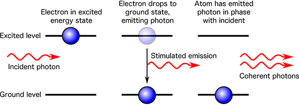
A laser is a device that emits light through a process known as stimulated emission. This occurs when a population of atoms exists in an excited energy state, meaning that the energy of one or more electrons in some of the atoms is not at the usual minimum energy state. In such a case, an electron can drop back down to the minimum energy state, emitting the excess energy as a photon of light; this is known as spontaneous emission. The stimulated emission part occurs when a photon interacts with another excited atom, triggering it to also drop into the minimum energy state and release a photon of the same energy. This stimulated photon is emitted in the same direction and with the same phase as the original photon (meaning the peaks and troughs of the light waves are in synch). As more emission is stimulated, an intense beam of light of a single wavelength, all travelling in the same direction is generated, known as a coherent beam.

Stimulated emission

Diagram of stimulated emission. The electron energy levels are within the confines of an atom (not shown).

Mechanically, this can be produced by using a transparent medium such as a gas or crystal, in a long cylinder shape surrounded by a bright strobe tube to supply the energy to excite the atoms. One end of the cylinder is a mirror, and the other end is a partly reflective mirror which lets some of the beam out. The light that emerges is a laser beam. Because the light is coherent, it doesn’t spread out like normal light, but travels in a tight line, illuminating only a small spot when it hits something. This means a laser beam is capable of travelling far greater distances than a normal light source of the same intensity, while still being bright enough to be observed.

Diagram of a laser

Diagram of a laser. (Modified from Creative Commons Attribution 3.0 Unported image by Matthew Leigh, from Wikimedia Commons.)

One of the very first applications for lasers was invented in 1961, but was restricted to industry and research for a decade. If you aim a brief laser pulse at something and time how long it takes for the reflection to come back, you can divide by the speed of light to calculate the distance to the object. This is called lidar, a portmanteau of “light” and “radar”, as it’s the same principle applied to light instead of radio waves. Lidar works to a range of several kilometres for detecting normal objects that partially reflect the incident beam.

But we can do a lot better if we construct a special target that reflects back virtually all of the incident beam. This can be done with a retroreflector. A common design is three flat mirrors arranged around a 90° corner, like the corner of a box. The combination of reflection off all three surfaces means that any incoming beam of light will be reflected back exactly towards its source, no matter what angle it comes in at. If you shine a laser at one of these, you can detect the return pulse over a much greater range. This form of lidar is known as laser ranging.

A corner retroreflector. No matter which direction incident light arrives from, the reflected beam returns in the same direction. (Public domain image from Wikimedia Commons.)

In 1964, NASA launched the Explorer 22 satellite into near-Earth orbit, about 1000 kilometres altitude. Its main mission was to perform science on the Earth’s ionosphere, but it was also equipped with a retroreflector, and was the first object in space to have its distance measured using satellite laser ranging.

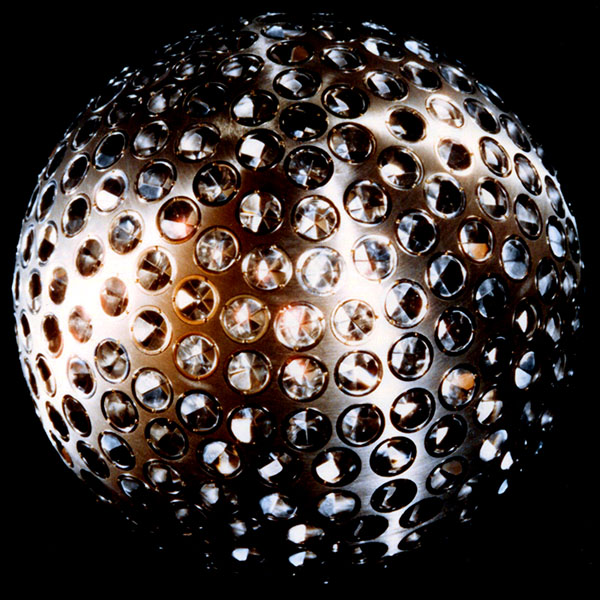
In 1976, NASA launched LAGEOS 1, a satellite designed specifically for laser ranging. LAGEOS has no active components, it is simply a brass sphere, coated in aluminium, with 426 retroreflectors embedded in the surface, so that no matter which way the satellite tumbles, dozens of reflectors are always oriented towards Earth.

Model of LAGEOS 1 satellite. (Public domain image by NASA, from nasa.gov.)

LAGEOS 1 is in medium-Earth orbit, at an altitude of nearly 6000 km. This orbit is far from any perturbing influences and so is extremely stable, meaning the satellite’s position at any time can be calculated to a small fraction of a millimetre. This makes it a useful reference point for measuring the distances to stations on the Earth’s surface, by aiming lasers at the satellite and timing the reflected signal.

Satellite laser ranging in action. Laser Ranging Facility at the Geophysical and Astronomical Observatory at NASA’s Goddard Spaceflight Center. The lasers are aimed at the Lunar Reconnaissance Orbiter, in orbit around the moon. (Public domain image by NASA from Wikimedia Commons.)

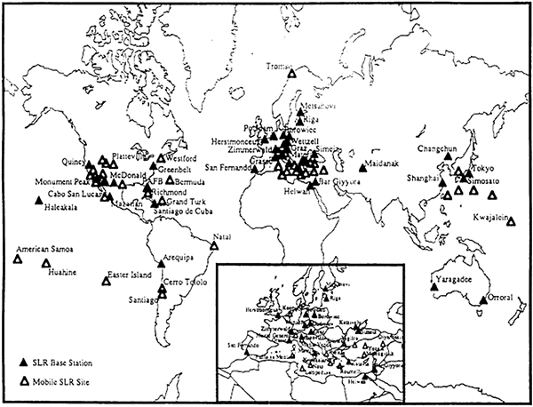
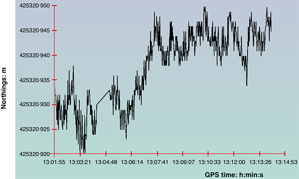
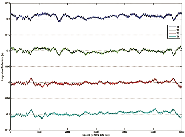
These measurements are so precise that they give the distance from the ground station to the satellite to an uncertainty of less than one millimetre. By using a reference point located away from Earth, this provides a method of checking motions of the Earth caused by weather systems, earthquakes, isostatic rebound (the slow rising of land in the millennia after glacial ice sheets melted), and tectonic drift. For example, geophysical tectonic modelling suggests that the Hawaiian Islands should be drifting northwards at approximately 70 mm per year. Measurement of the position of the Haleakala laser base station in Hawaii using LAGEOS and similar satellites shows this to be the case.

Laser ranging stations worldwide

Satellite laser ranging stations around the world. (Figure reproduced from [1].)

Laser ranging can also be (and is) used to measure the shape of the Earth. More specifically, it’s used to measure the shape of the geoid, which is the shape that corresponds to mean sea level (averaging out tides and weather) all over the Earth. More formally this is defined as the surface where the Earth’s gravitational field strength is identical to that at sea level. In areas of land, this surface is generally under the ground. The geoid is not perfectly spherical due to the uneven distribution of mass in the Earth. We’ve mentioned a few times that the Earth is approximately an ellipsoid due to the rotational force flattening the poles and causing a bulge at the equator. The geoid is almost an ellipsoid, but varies locally by up to approximately ±100 metres.

The geoid surface relative to an ellipsoid, shown as highly exaggerated relief. The darkest blue area below India is -106 m, while the red area near Iceland is +85 m. (Creative Commons Attribution 4.0 International image by the International Centre for Global Earth Models, from Wikimedia Commons.)

Besides LAGEOS 1 and 2, there are a handful of other similar retroreflector satellites. And there are also retroreflectors on the moon. Astronauts on NASA’s Apollo 11, 14, and 15 missions set up retroreflector arrays on the moon’s surface, and the unmanned Russian probes Lunakhod 1 and 2 also have retroreflectors.

Retroreflector array set up on the lunar surface by Neil Armstrong and Buzz Aldrin during the Apollo 11 mission. (Public domain image by NASA from Wikimedia Commons.)

Since 1969, several lunar laser ranging experiments have been ongoing, making regular measurements of the distance between the Earth stations and the reflectors on the moon. These measurements can also determine the distance to better than one millimetre.

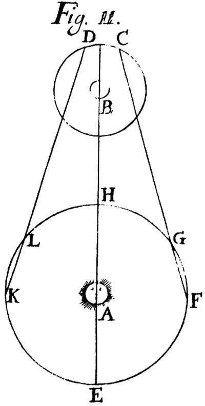
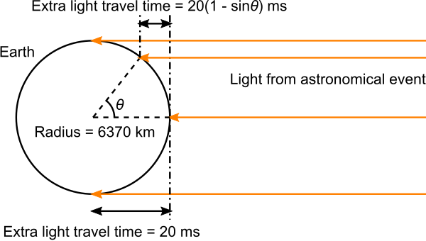
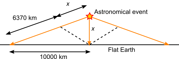
If you measure the distances from either an artificial satellite or the moon to different points on the Earth’s surface, it’s trivial to show that the points don’t lie even approximately on a flat plane, but that they lie on the surface of an approximately spherical body with the radius of the Earth. Finding an explicit statement such as “This demonstrates that the Earth is not flat, but spherical” in a published scientific article is difficult (because that result is neither surprising nor groundbreaking), but the following diagram shows the model that laser ranging scientists use to correct for effects such as atmospheric refraction, to enable them to get their measurements accurate down to a millimetre.

Model of Earth used for accurate laser ranging

Atmospheric refraction model used by laser ranging scientists. (Figure reproduced from [1].)

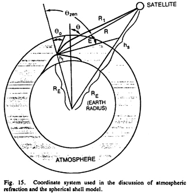
This shows clearly that laser ranging scientists—who have explicit and direct measurements of the shape of the Earth’s surface—assume the Earth is spherical in order to refine their calculations. They’d hardly do that if the Earth were flat.

References:

[1] Degnan, J. J. “Millimeter accuracy satellite laser ranging: a review”. Contributions of Space Geodesy to Geodynamics: Technology, 25, p.133-162, 1993. https://doi.org/10.1029/GD025p0133

[2] Murphy Jr., T. W. “Lunar Laser Ranging: The Millimeter Challenge”. Reports on Progress in Physics, 76(7), p. 076901, 2013. https://doi.org/10.1088/0034-4885/76/7/076901

19. Bridge towers

When architects design and construction engineers build towers, they make them vertical. By “vertical” we mean straight up and down or, more formally, in line with the direction of gravity. A tall, thin structure is most stable if built vertically, as then the centre of mass is directly above the centre of the base area.

If the Earth were flat, then vertical towers would all be parallel, no matter where they were built. On the other hand, if the Earth is curved like a sphere, then “vertical” really means pointing towards the centre of the Earth, in a radial direction. In this case, towers built in different places, although all locally vertical, would not be parallel.

The Humber Bridge spans the Humber estuary near Kingston upon Hull in northern England. The Humber estuary is very broad, and the bridge spans a total of 2.22 kilometres from one bank to the other. It’s a single-span suspension bridge, a type of bridge consisting of two tall towers, with cables strung in hanging arcs between the towers, and also from the top of each tower to anchor points on shore. (It’s the same structural design as the more famous Golden Gate Bridge in San Francisco.) The cables extend in both directions from the top of each tower to balance the tension on either side, so that they don’t pull the towers over. The road deck of the bridge is suspended below the main cables by thinner cables that hang vertically from the main cables. The weight of the road deck is thus supported by the main cables, which distribute the load back to the towers. The towers support the entire weight of the bridge, so must be strong and, most importantly, exactly vertical.

The Humber Bridge from the southern bank of the Humber. (Public domain image from Wikimedia Commons.)

The towers of the Humber Bridge rest on pylons in the estuary bed. The towers are 1410 metres apart, and 155.5 metres high. If the Earth were flat, the towers would be parallel. But they’re not. The cross-sectional centre lines at the tops of the two towers are 36 millimetres further apart than at the bases. Using similar triangles, we can calculate the radius of the Earth from these dimensions:

Radius = 155.5×1410÷0.036 = 6,090,000 metres

This gives the radius of the Earth as 6100 kilometres, close to the true value of 6370 km.

Size of the Earth from the Humber Bridge

Diagram illustrating use of similar triangles to determine the radius of the Earth from the Humber Bridge data. (Not to scale!)

If this were the whole story, it would pretty much be case closed at this point. However, despite a lot of searching, I couldn’t find any reference to the distances between the towers of the Humber Bridge actually being measured at the top and the bottom. It seems that the figure of 36 mm was probably calculated, assuming the curvature of the Earth, which makes this a circular argument (pun intended).

Interestingly, I did find a paper about measuring the deflection of the north tower of the Humber Bridge caused by wind loading and other dynamic stresses in the structure. The paper is primarily concerned with measuring the motion of the road deck, but they also mounted a kinematic GPS sensor at the top of the northern tower[1].

GPS sensor on Humber Bridge north tower

Kinematic GPS sensor mounted on the top of the north tower of the Humber Bridge. (Reproduced from [1].)

The authors carried out a series of measurements, and show the results for a 15 minute period on 7 March, 1996.

Deflections of Humber Bridge north tower

North-south deflection of the north tower of the Humber Bridge over a 15 minute period. The vertical axis is metres relative to a standard grid reference, so the full vertical range of the graph is 30 mm. (Reproduced from [1].)

From the graph, we can see that the tower wobbles a bit, with deflections of up to about ±10 mm from the mean position. The authors report that the kinematic GPS sensors are capable of measuring deflections as small as a millimetre or two. So from this result we can say that the typical amount of flexing in the Humber Bridge towers is smaller than the supposed 36 mm difference that we should be trying to measure. So, in principle, we could measure the fact that the towers are not parallel, even despite motion of the structure in environmental conditions.

A similar result is seen with the Severn Bridge, a suspension bridge over the Severn River between England and Wales. It has a central span of 988 metres, with towers 136 metres tall. A paper reports measurements made of the flexion of both towers, showing typical deflections at the top are less than 10 mm[2].

Deflections of Severn Bridge towers

Plot of deflection of the top of the suspension towers along the axis of the Severn Bridge. T1 and T2 (upper two lines) are measurements made by two independent sensors at the top of the west tower; T3 and T4 (lower lines) are measurements made by sensors on the east tower. Deflection is in units of metres, so the scale of the maximum deflections is about 10 mm. (Reproduced from [2].)

Okay, so we could in principle measure the mean positions of the tops of suspension bridge towers with enough precision to establish that the towers are further apart at the top than the base. A laser ranging system could do this with ease. Unfortunately, in all my searching I couldn’t find any citations for anyone actually doing this. (If anyone lives near the Humber Bridge and has laser ranging equipment, climbing gear, a certain disregard for authority, and a deathwish, please let me know.)

Something I did find concerned the Verrazzano-Narrows Bridge in New York City. It has a slightly smaller central span than the Humber Bridge, with 1298 metres between its two towers, but the towers are taller, at 211 metres. The tops of the towers are reported as being 41.3 mm further apart than the bases, due to the curvature of the Earth. There are also several citations backing up the statement that “the curvature of the Earth’s surface had to be taken into account when designing the bridge” (my emphasis).[3]

Verrazzano-Narrows Bridge, linking Staten Island (background) and Brooklyn (foreground) in New York City. (Public domain image from Wikimedia Commons.)

So, this prompts the question: Do structural engineers really take into account the curvature of the Earth when designing and building large structures? The answer is—of course—yes, otherwise the large structures they build would be flawed.

There is a basic correction listed in The Engineering Handbook (published by CRC) to account for the curvature of the Earth. Section 162.5 says:

The curved shape of the Earth… makes actual level rod readings too large by the following approximate relationship: C = 0.0239 D² where C is the error in the rod reading in feet and D is the sighting distance in thousands of feet.[4]

To convert to metric we need to multiply the constant by the number of feet in a metre (because of the squared factor), giving the correction in metres = 0.0784×(distance in km)². What this means is that over a distance of 1 kilometre, the Earth’s surface curves downwards from a perfectly straight line by 78.4 millimetres. This correction is well known among civil and structural engineers, and is applied in surveying, railway line construction, bridge construction, and other areas. It means that for engineering purposes you can’t treat the Earth as both flat and level over distances of around a kilometre or more, because it isn’t. If you treat it as flat, then a kilometre away your level will be off by 78.4 mm. If you make a surface level (as measured by a level or inclinometer at each point) over a kilometre, then the surface won’t be flat; it will be curved parallel to the curvature of the Earth, and 78.4 mm lower than flat at the far end.

An example of this can be found at the Volkswagen Group test track facility near Ehra-Lessien, Germany. This track has a circuit of 96 km of private road, including a precision level-graded straight 9 km long. Over the 9 km length, the curvature of the Earth drops away from flat by 0.0784×9² = 6.35 metres. This means that if you stand at one end of the straight and someone else stands at the other end, you won’t be able to see each other because of the bulge of the Earth’s curvature in between. The effect can be seen in this video[5].

One set of structures where this difference was absolutely crucial is the Laser Interferometer Gravitational-Wave Observatory (LIGO) constructed at two sites in Hanford, Washington, and Livingston, Louisiana, in the USA.

The LIGO site at Hanford, Washington. Each of the two arms of the structure are 4 km long. (Public domain image from Wikimedia Commons.)

LIGO uses lasers to detect tiny changes in length caused by gravitational waves from cosmic sources passing through the Earth. The lasers travel in sealed tubes 4 km long, which are under high vacuum. Because light travels in a straight line in a vacuum, the tubes must be absolutely straight for the machine to work. The tubes are level in the middle, but over the 2 km on either side, the curvature of the Earth falls away from a straight line by 0.0784×2² = 0.314 metres. So either end of the straight tube is 314 mm higher than the centre of the tube. To build LIGO, they laid a concrete foundation, but they couldn’t make it level over the distance; they had to make it straight. This required special construction techniques, because under normal circumstances (such as Volkswagen’s track at Ehra-Lessien) you want to build things level, not straight.[6]

So, the towers of large suspensions bridges almost certainly are not parallel, due to the curvature of the Earth, although it seems nobody has ever bothered to measure this. But it’s certainly true that structural engineers do take into account the curvature of the Earth for large building projects. They have to, because if they didn’t there would be significant errors and their constructions wouldn’t work as planned. If the Earth were flat they wouldn’t need to do this and wouldn’t bother.

UPDATE 2019-07-10: NASA’s Jet Propulsion Laboratory has announced a new technique which they can use to detect millimetre-sized shifts in the position of structures such as bridges, using aperture synthesis radar measurements from satellites. So maybe soon we can have more and better measurements of the positions of bridge towers![7]

References:

[1] Ashkenazi, V., Roberts, G. W. “Experimental monitoring of the Humber bridge using GPS”. Proceedings of the Institution of Civil Engineers – Civil Engineering, 120, p. 177-182, 1997. https://doi.org/10.1680/icien.1997.29810

[2] Roberts, G. W., Brown, C. J., Tang, X., Meng, X., Ogundipe, O. “A Tale of Five Bridges; the use of GNSS for Monitoring the Deflections of Bridges”. Journal of Applied Geodesy, 8, p. 241-264, 2014. https://doi.org/10.1515/jag-2014-0013

[3] Wikipedia: “Verrazzano-Narrows Bridge”, https://en.wikipedia.org/wiki/Verrazzano-Narrows_Bridge, accessed 2019-06-30. In turn, this page cites the following sources for the statement that the curvature of the Earth had to be taken into account during construction:

[3a] Rastorfer, D. Six Bridges: The Legacy of Othmar H. Ammann. Yale University Press, 2000, p. 138. ISBN 978-0-300-08047-6.

[3b] Caro, R.A. The Power Broker: Robert Moses and the Fall of New York. Knopf, 1974, p. 752. ISBN 978-0-394-48076-3.

[3c] Adler, H. “The History of the Verrazano-Narrows Bridge, 50 Years After Its Construction”. Smithsonian Magazine, Smithsonian Institution, November 2014.

[3d] “Verrazano-Narrows Bridge”. MTA Bridges & Tunnels. https://new.mta.info/bridges-and-tunnels/about/verrazzano-narrows-bridge, accessed 2019-06-30.

[4] Dorf, R. C. (editor). The Engineering Handbook, Second Edition, CRC Press, 2018, ISBN 978-0-849-31586-2.

[5] “Bugatti Veyron Top Speed Test”. Top Gear, BBC, 2008. https://youtu.be/LO0PgyPWE3o?t=200, accessed 2019-06-30.

[6] “Facts about LIGO”, LIGO Caltech web site. https://www.ligo.caltech.edu/page/facts, accessed 2019-06-30.

[7] “New Method Can Spot Failing Infrastructure from Space”, NASA JPL web site. https://www.jpl.nasa.gov/news/news.php?feature=7447, accessed 2019-07-10.

17. Light time corrections

In the 16th century, the naval powers of Europe were engaged in a race to explore and colonise lands previously unknown to Europeans (though many were of course already inhabited), and reap the rewards of the new found resources. They were limited by the accuracy of navigation at sea. Determining latitude was a relatively simple matter of sighting the angle of a star or the sun through a sextant. But because of the daily rotation of the Earth, determining the longitude by sighting a celestial object required knowing the time of day. Mechanical clocks of the era were rendered useless by the rocking of a ship, making this a major problem.

Solving the problem would give such an advantage to the country holding the secret that in 1598 King Philip III of Spain offered a prize of 6000 ducats plus an annual pension of 2000 ducats for life to whoever could devise a means of measuring longitude at sea. In 1610 the prize was still unclaimed, and in that year Galileo Galilei trained his first telescope on Jupiter, becoming the first person to observe the planet’s largest four moons. He studied their movements, and a couple of years later had produced orbital tables that allowed their positions to be calculated months or years in advance. These tables included the times when a moon would slip into Jupiter’s shadow, and be eclipsed, disappearing from view because it no longer reflected sunlight.

Galileo wrote to King Philip in 1616, proposing a method of telling the time at sea by observing the eclipses of Jupiter’s moons. One could pinpoint the time by observing an eclipse, and then use an observation of a star to calculate the longitude. Although the method could work in principle, observing an eclipse of a barely visible object through the narrow field of view of a telescope while standing on a rocking ship was practically impossible, and it never worked in practice.

Jupiter and its innermost large moon, Io, as seen by NASA’s Cassini space probe. (Galileo’s view was nowhere near as good as this!) (Public Domain image by NASA.)

By the 1660s, Giovanni Cassini had developed Galileo’s method as a way of measuring precise longitudes on land, as an aid to calculating distances and making accurate maps. In 1671 Cassini moved to take up directorship of the Royal Observatory in Paris. He dispatched his assistant Jean Picard to Uraniborg, the former observatory of Tycho Brahe, near Copenhagen, partly to make measurements of eclipses of Jupiter’s moon Io, to accurately calculate the longitude difference between the two observatories. Picard himself employed the assistance of a young Dane named Ole Rømer.

Portrait of Ole Rømer by Jacob Coning. (Public domain image from Wikimedia Commons.)

The moon Io orbits Jupiter every 42.5 hours and is close enough to be eclipsed on each orbit, so an eclipse is visible every few days, weather and daylight hours permitting. After observing well over 100 eclipses, Rømer moved to Paris to assist Cassini himself, and continued recording eclipses of Io over the next few years. In these observations Cassini noticed some odd discrepancies. In particular, the time between successive eclipses got shorter when the Earth was approaching Jupiter in its orbit, and longer several months later when the Earth was moving away from Jupiter. Cassini realised that this could be explained if the light from Io did not arrive at Earth instantaneously, but rather took time to travel the intervening distance. When the Earth is closer to Jupiter, the light has less distance to cover, so the eclipse appears to occur earlier, and vice versa: when the Earth is further away the eclipse appears to be later because the light takes longer to reach Earth. Cassini made an announcement to this effect to the French Academy of Sciences in 1676.

Ole Rømer’s notebook showing recordings of the dates and times of eclipses of Io from 1667 to 1677. “Imm” means immersion into Jupiter’s shadow, and “Emer” means emergence from Jupiter’s shadow. (Public domain image from Wikimedia Commons.)

However, it was common wisdom at the time that light travelled instantaneously, and Cassini later retreated from his suggestion and did not pursue it further. Rømer, on the other hand, was intrigued and continued to investigate. In 1678 he published his findings. He argued that as the Earth moved in its orbit away from Jupiter, successive eclipses would each occur with the Earth roughly 200 Earth-diameters further away from Jupiter than the previous one. Using the geometry of the orbit and his observations, Rømer calculated that it must take light approximately 11 minutes to cross a distance equal to the diameter of the Earth’s orbit. This is a little low—it actually takes about 16 and a half minutes—but it’s the right order of magnitude. So for the first time, we had some idea how fast light travels. And as we’ve just seen, the finite speed of light can have a significant effect on the observed timing of astronomical observations.

Ole Rømer's figure

Figure 2 from Rømer’s paper, illustrating the difference in distance between Earth and Jupiter between successive eclipses as Earth recedes from Jupiter (LK) and approaches Jupiter (FG). Reproduced from [1].

The finite speed of light means that astronomical events don’t occur when we see them. We only see the event after enough time has elapsed for the light to travel to Earth. This is important for events with precisely measurable times, such as eclipses, occultations, the brightness variations of variable stars, and the radio pulses of remote pulsars.

Not only do you need to correct for the time it takes light to reach Earth, but the correction is different depending on where you are on Earth. An observer observing an object that is directly overhead is closer to it than an observer seeing the same object on the horizon. The observer seeing the object on the horizon is further away by the radius of the Earth. The radius of the Earth is 6370 km, and it takes light a little over 21 milliseconds to travel this distance. So astronomical events observed on the horizon appear to occur 21 milliseconds later than they do to someone observing the same event overhead. This effect is significant enough to be mentioned explicitly in a paper discussing the timing of variable stars:

“More disturbing effects become significant which require more conventions and more complex reduction procedures. By far the biggest effect is the topocentric light-time correction (up to 20 msec).”[2]

Topocentric refers to measuring from a specific point on the surface of the Earth. Depending where on Earth you are, the timing of observed astronomical events can appear to vary by up to 20 ms.

Not only does the light travel time affect the observed time of astronomical events, it also affects the observed position of some astronomical objects, most importantly solar system objects that move noticeably over the few hours that light takes to travel to Earth from them. When we observe an object such as a planet or an asteroid, we see it in the position that it was when the light left it, not where it is at the time that we see it. So for such objects, a corrected position needs to be calculated. The correction in observed position of a moving astronomical object due to the finite speed of light is, somewhat confusingly, also known as light time correction.

Light time correction of observed position is critical in determining the orbits of bodies such as asteroids and comets with accuracy. A paper describing general methods for determining orbital parameters from observations notes that Earth-based observations are necessarily topocentric, and states in the description of the method that:

“In the case of asteroid or comet orbits, the light-time correction has been computed.”[3]

Finally, a recent paper on determining the orbital parameters of near-Earth objects (which pose a potential threat of catastrophic collision with Earth) points out, where ρ is the topocentric distance:

“Note that we include a light-time correction by subtracting ρ/c from the observed epochs for any propagation computation with c as speed of light.”[4]

All of these corrections, which must be applied to astronomical observations where either (a) timings must be known to less than a second or (b) positions must be known accurately to determine orbits, are different by a light travel time of 21 ms for observers looking at objects directly overhead versus observers looking towards the horizon. And in between the light time corrections are 21 ms × (1 minus the sine of the observation zenith angle).

light time corrections on a spherical Earth

Diagram of light time corrections. Observation points where an astronomical event are on the horizon are 6370 km further away than observation points where the event is directly overhead.

This implies that places on Earth where an astronomical object appears near the horizon are a bit over 6000 km further away from the object than the location where the object is directly overhead. This is true no matter which object is observed, meaning it is independent of which position on Earth is directly under it. This cannot be so if the Earth is flat.

light time corrections on a flat Earth

Geometry of light time corrections on a flat Earth.

Observation points on Earth where an astronomical event is overhead and on the horizon are separated by 10,000 km. If the Earth is flat, then the geometry must be something like that shown in the diagram above. The astronomical event is a distance x above the flat Earth, such that the distance from the event to a point 10,000 km along the surface is x plus the measured light travel time distance of 6370 km. Applying Pythagoras’s theorem:

(6370 + x)² = 10000² + x²

Solving for x gives 4660 km. So measurements of light time correction imply that all astronomical events are 4660 km above the flat Earth. This means the elevation angle of the event seen from 10,000 km away is arctan(4660/10,000) = 25°, well above the horizon, which is inconsistent with observation (and the trigonometry of all the intermediate angles doesn’t work either). It’s also easy to show by other observations that astronomical objects are not all at the same distance – some are thousands, millions, or more times further away than others, and they are all much further away than 4660 km.

So the measurement of light time corrections imply that observers on Earth are positioned on the surface of a sphere. In other words, that the Earth is spherical in shape.

References:

[1] Rømer, O. (“A Demonstration Concerning the Motion of Light”.) Philosophical Transactions of the Royal Society, 12, p. 893-94, 1678. (Originally published in French as “Demonstration touchant le mouvement de la lumiere trouvé”. Journal des Sçavans, p. 276-279, 1677.) https://www.jstor.org/stable/101779

[2] Bastian, U. “The Time Coordinate Used in the Variable-star Community”. Information Bulletin on Variable Stars, No. 4822, #1, 2000. https://ui.adsabs.harvard.edu/abs/2000IBVS.4822….1B/abstract

[3] Dumoulin, C. “Unified Iterative Methods in Orbit Determination”. Celestial Mechanics and Dynamical Astronomy, 59, 1, p. 73-89, 1994. https://doi.org/10.1007/BF00691971

[4] Frühauf, M., Micheli, M., Santana-Ros, T., Jehn, R., Koschny, D., Torralba, O. R. “A systematic ranging technique for follow-ups of NEOs detected with the Flyeye telescope”. Proceedings of the 1st NEO and Debris Detection Conference, Darmstadt, 2019. https://ui.adsabs.harvard.edu/abs/2019arXiv190308419F/abstract

10. The Sagnac effect

Imagine beams of light coming from an emitter and travelling around a circular path in both directions, until they arrive back at the source. Such an arrangement can be constructed by using an optic fibre in a circular loop, injecting light at both ends. The distance travelled by the clockwise beam is the same as the distance travelled by the anticlockwise beam, and the speed of light in both directions is the same, so the time taken for each beam to travel from the source back to the origin is the same. So far, so good.

A light loop

A loop with light travelling in both directions.

Now imagine the whole thing is rotating – let’s say clockwise. For reference we’ll use the numbers on a clock face and the finer divisions into 60 minutes. The optic fibre ring runs around the edge of the clock, with the light source and a detector at 12. Now imagine that the clock rotates fast enough that by the time the clockwise-going light reaches the original 12 position, the clock has rotated so that 12 is now located at the original 1 minute past 12 position. The light has to travel an extra 60th of the circle to reach its starting position (actually a tiny bit more than that because the clock is still rotating and will have gone a tiny bit further by the time the light beam catches up). But the light going anticlockwise reaches the source early, only needing to travel a tiny bit more than 59/60 of the circle. The travel times of the two beams of light around the circle are different.

A rotating light loop

Now the loop is rotating. By the time the light has travelled around the loop, the exit from the loop has moved a little bit clockwise. So the light travelling clockwise has to travel further to reach the exit, while the light travelling anticlockwise reaches the exit sooner.

This is a very simplified explanation, and figuring out the mathematics of exactly what happens involves using special relativity, since the speed of light is involved, but it can be shown that there is indeed a time difference between the travel times of beams of light heading in opposite directions around a rotating loop. The time difference is proportional to the speed of rotation and to the area of the loop (and to the cosine of the angle between the rotation axis and the perpendicular to the loop, for those who enjoy vector mathematics). This effect is known as the Sagnac effect, named after French physicist Georges Sagnac, who first demonstrated it in 1913.

Measuring the minuscule time difference between the propagation of the light beams is not difficult, due to the wave nature of light itself. The wavelength of visible light is just a few hundred nanometres, so even a time difference of the order of 10^-16 seconds can be observed because it moves the wave crests and troughs of the two beams relative to one another, causing visible interference patterns as they shift out of synchronisation. This makes the device an interferometer that is very sensitive to rotational speed.

The Sagnac effect can be seen not only in a circular loop of optic fibre, but also with any closed loop of light beams of any shape, such as can be constructed with a set of mirrors. This was how experimenters demonstrated the effect before the invention of optic fibres. Because the paths of the two beams of light are the same, just reversed, a Sagnac interferometer is completely insensitive to mechanical construction tolerances, and only sensitive to the physical rotation of the device.

Sagnac actually performed the experiment in an attempt to prove the existence of the luminiferous aether, a hypothetical medium permeating all space through which light waves propagate. He believed his results showed that such an aether existed, but Max von Laue and Albert Einstein showed that Sagnac’s effect could be explained by special relativity, without requiring any aether medium for light propagation.

The interesting thing about the Sagnac effect is that it measures absolute rotational speed, that is: rotation relative to an inertial reference frame, in the language of special relativity. In practice, this means rotation relative to the “fixed” position of distant stars. This is useful for inertial guidance systems, such as those found on satellites, modern airliners and military planes, and missiles. The Sagnac effect is used in ring laser gyroscopes and fibre optic gyroscopes to provide an accurate measure of rotational speed in these guidance systems. GPS satellites use these devices to ensure their signals are correctly calibrated for rotation – without them GPS would be less accurate.

Because the magnitude of the Sagnac effect depends on both the rotational speed and the area of the light loop, by making the area large you can make the interferometer incredibly sensitive to even very slow rotation. Rotations as slow as once per 24 hours. You can use these devices to measure the rotation of the Earth.

This was first done in 1925. Albert A. Michelson (of the famous Michelson-Morley experiment that disproved the existence of the luminiferous aether), Henry G. Gale, and Fred Pearson acquired the use of a tract of land in Clearing, Illinois (near Chicago’s Midway Airport), and built a huge Sagnac interferometer, a rectangle 610×340 metres in size [1][2].

Michelson’s Sagnac interferometer

Diagram of Michelson’s Sagnac interferometer in Clearing, Illinois. The Sagnac loop is defined by the mirrors ADEF. The smaller rectangle ABCD was used for calibration measurements. Light enters from the bottom towards the mirror A, which is half-silvered, allowing half the light through to D, and reflecting half in the other direction towards F. The beams complete circuits ADEF and AFED, returning to A, where the half-silvering reflects the beam from D and lets through the beam from F towards the detector situated outside the loop at the left. The light paths are inside a pipe system, which is evacuated using a pump to remove most of the air. (Figure reproduced from [2].)

With this enormous area, the shift in the light beams caused by the rotation speed of the Earth at the latitude of Chicago was around one fifth of a wavelength of the light used – easily observable. The Michelson-Gale-Pearson experiment’s measurements and calculations showed that the rotation speed they measured was consistent with the rotation of the Earth once every 23 hours and 56 minutes – a sidereal day (i.e. Earth’s rotation period relative to the stars; this is shorter than the average of 24 hours rotation relative to the sun, because the Earth also moves around the sun).

Now the interesting thing is that the Sagnac effect measures the linear rotation speed, not the angular rotation rate. The Earth rotates once per day – that angular rotation rate is constant for the entire planet, and can be modelled in a flat Earth model simply by assuming the Earth is a spinning disc, like a vinyl record or Blu-ray disc. But the linear rotation speed of points on the surface of the Earth varies.

In the typical flat Earth model with the North Pole at the centre of the disc, the rotation speed is zero at the North Pole, and increases linearly with distance from the Pole. As you cross the equatorial regions, the rotational speed just keeps increasing linearly, until it is maximal in regions near the “South Pole” (wherever that may be).

Rotation speed on a flat disc Earth

Rotation speeds at different places on a flat rotating disc Earth (top view of the disc).

On a spherical Earth, in contrast, the rotation speed is zero at the North Pole, and varies as the cosine of the latitude as you travel south, until it is a maximum at the equator, then drops again to zero at the South Pole.

Rotation speed on a flat disc Earth

Rotation speeds at different places on a spherical Earth.

Here is a table of rotation speeds for the two models:

Latitude	Speed (km/h) Flat model	Speed (km/h) Spherical model
90°N (North Pole)	0.0	0.0
60°N	875.3	837.2
41.77°N (Clearing, IL)	1407.2	1248.9
30°N	1750.5	1450.1
0° (Equator)	2625.8	1674.4
30°S	3501.1	1450.1
45.57°S (Christchurch)	3896.6	1213.3
60°S	4376.4	837.2
90°S (South Pole)	5251.6	0.0

In the Michelson-Gale-Pearson experiment, the calculated expected interferometer shift was 0.236±0.002 of a fringe (essentially a wavelength of the light used), and the observed shift was 0.230±0.005 of a fringe. The uncertainty ranges overlap, so the measurement is consistent with the spherical Earth model that they used to calculate the expected result.

If they had used the North-Pole-centred flat Earth model, then the expected shift would have been 1407.2/1248.9 larger, or 0.266±0.002 of a fringe. This is well outside the observed measurement uncertainty range. So we can conclude that Michelson’s original 1925 experiment showed that the rotation of the Earth is inconsistent with the flat Earth model.

Nowadays we have much more than that single data point. Sagnac interferometers are routinely used to measure the rotation speed of the Earth at various geographical locations. In just one published example, a device in Christchurch, New Zealand, at a latitude of 43°34′S, measured the rotation of the Earth equal to the expected value (for a spherical Earth) to within one part in a million [3]. Given that the expected flat Earth model speed is more than 3 times the spherical Earth speed at this latitude—and all of the other rotation speed measurements made all over the Earth consistent with a spherical Earth—we can well and truly say that any rotating disc flat Earth model is ruled out by the Sagnac effect.

References:
[1] Michelson, A. A. “The Effect of the Earth’s Rotation on the Velocity of Light, I.” The Astrophysical Journal, 61, 137-139, 1925. https://doi.org/10.1086%2F142878
[2] Michelson, A. A.; Gale, Henry G. “The Effect of the Earth’s Rotation on the Velocity of Light, II.” The Astrophysical Journal, 61, p. 140-145, 1925. https://doi.org/10.1086%2F142879
[3] Anderson, R.; Bilger, H. R.; Stedman, G. E. “ “Sagnac” effect: A century of Earth‐rotated interferometers”. American Journal of Physics, 62, p. 975-985, 1994. https://doi.org/10.1119/1.17656

Share this:

Share this:

Share this:

Share this: