geology – 100 Proofs that the Earth is a Globe

39. Seismic wave propagation

Our planet is made largely of rocks and metals. The composition and physical state varies with depth from the core of the Earth to the surface, because of changes in pressure and temperature with depth. The uppermost layer is the crust, which consists of lighter rocks in a solid state. Immediately below this is the upper mantle, in which the rocks are hotter and can deform plasticly over millions of years.

Slow convection currents occur in the upper mantle, and the convection cells define the tectonic plates of the Earth’s crust. Where mantle material rises, magma can emerge at mid-oceanic ridges or volcanoes. Where it sinks, a subduction zone occurs in the crust.

The plate boundaries are thus particularly unstable places on the Earth. As the plates shift and move relative to one another, stresses build up in the rock along the edges. At some point the stress becomes too great for the rock to withstand, and it gives way suddenly, releasing energy that shakes the Earth locally. These are earthquakes.

Engraving of the effects of the 1755 Lisbon earthquake. (Public domain image from Wikimedia Commons.)

The point of slippage and the release of energy is known as the hypocentre of the earthquake, and may be several kilometres deep underground. The point on the surface above the hypocentre is the epicentre, and is where potential destruction is the greatest. Most earthquakes are small and go relatively unnoticed except by the seismologists who study earthquakes. Sometimes a quake is large and can cause damage to structures, injuries, and loss of life.

The energy released in an earthquake travels through the Earth in the form of waves, known as seismic waves. There are a few different types of seismic wave.

Primary waves, or P waves, are compressional waves, like sound waves in air. The rock alternately compresses and experiences tension, in a direction along the axis of propagation. In fact P waves are essentially sound waves of very large amplitude, and they propagate at the speed of sound in the medium. Within surface rock, this is about 5000 metres per second. Primary waves are so called because they are the fastest seismic waves, and thus the first ones to reach seismic recording stations located at any distance from the epicentre. They travel through the body of the Earth. And like sound waves, they can travel through any medium: solid, liquid, or gas.

Secondary waves, or S waves, are transverse waves, like light waves, or waves travelling along a jiggled rope. The rock jiggles from side to side as the wave propagates perpendicular to the jiggling motions. S waves travel a little over half the speed of P waves, and are the second waves to be detected at remote seismic stations. S waves also travel through the body of the Earth, but only within solid material. Fluids have no shear strength, and so cannot return to an equilibrium position when a transverse wave hits it, so the energy is dissipated within the fluid.

Seismic wave types

Illustrations of rock movement in different types of seismic waves. (Figure reproduced from [1].)

Besides these two types of body waves, there are also surface waves, which travel along the surface of the Earth. One type, Rayleigh waves (or R waves, named after the physicist Lord Rayleigh), are just like the surface waves or ripples on water, and causes the surface of the Earth to heave up and down. Another type of surface wave causes side to side motion; these are known as Love waves (or L waves, named after the mathematician Augustus Edward Hough Love). These waves propagate more slowly than S waves, at around 90% of the speed. Love waves are generally the strongest and most destructive seismic waves.

The P and S waves are thus the first two waves detected from an earthquake, and they are easily distinguishable on seismometer recordings.

Seismogram of P and S waves

Seismogram recording of arrival of P waves and S waves at a seismology station in Mongolia, from an earthquake 307 km away. (Figure reproduced from [2].)

The P waves arrive first and produce a pulse of activity which slowly fades in amplitude, then the S waves arrive and cause a larger amplitude burst of activity. Because the relative speeds of the two waves through the same material are known, the time between the arrival of the P and S waves can be used to determine the distance from the seismic station to the earthquake hypocentre, using a graph such as the following:

Seismic wave travel-time curves for P, S, and L waves. Also shown are three seismograms detected at seismic stations at different distances from an earthquake. (Public domain image from the United States Geological Survey.)

The graph shows the travel times of P, S, and also L waves, plotted against distance from the earthquake on the vertical axis. As you can see, the time between the detection of the P and S waves increases steadily with the distance from the quake.

If you have three seismic stations, you can triangulate the location of the epicentre (using trilateration, as we have previously discussed).

Triangulating the location of an earthquake using distances from three seismic stations. (Public domain image from United States Geological Survey.)

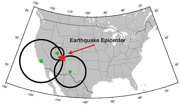
Of course, if you have more than three seismic stations, you can pinpoint the location of the earthquake much more reliably and precisely. According to the International Registry of Seismograph Stations, there are over 26,000 seismic stations around the world.

Location of seismic stations

Location of seismic stations recorded in the International Registry of Seismograph Stations. (Figure reproduced from [3].)

Interestingly, notice how the world’s seismic stations are concentrated along plate boundaries, where earthquakes are most common, particularly around the Pacific rim, as well as heavily in the developed nations of the US and Europe.

As shown in the travel-time curve graph, you can also use the propagation time of L waves to estimate distance to the earthquake. Did you notice the difference between the shapes of the P and S wave curves, and the L wave curve? L waves travel along the surface of the Earth. The distance from an earthquake to a detection station is measured conventionally, like everyday distances, also along the surface of the Earth. Since the L waves propagate at a constant speed, the graph of distance (along the Earth’s surface) versus time is a straight line.

But the P and S waves don’t travel along the surface of the Earth. They propagate through the bulk of the Earth. The distance that a P or S wave needs to travel from earthquake to detection site increases more slowly than the distance along the surface of the Earth, because of the Earth’s spherical shape. The S waves are only about 10% faster than the L waves, and you can see that near the epicentre, they arrive only around 10% earlier than the L waves. But the further away the earthquake is, the more of a shortcut they can take through the Earth, and so the faster they arrive, resulting in the downward curve on the graph. Similarly for the P waves.

This is in fact not the only cause of the P and S waves appearing to get faster the further away you are from an earthquake. They actually do get faster as they travel deeper, because of changes to the rock pressure. Deep in the Earth they can travel at roughly twice the speed that they do near the surface. The combination of these effects causes the shape of the curves in the travel-time graph.

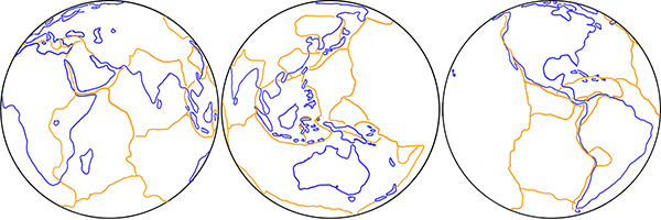
If we consider the propagation of seismic waves from an earthquake, they spread out in circles around the epicentre, like ripples in a pond from where a stone is dropped in. The arrival times of the waves at seismic stations equidistant from the epicentre should be the same, since the speeds in any direction are the same. And this is of course what is observed. The following figures show the predicted spread of P waves across the Earth from earthquake epicentres in Washington State USA, near Panama, and near Ecuador, as plotted by the US Geological Survey.

P wave propagation times from Washington

Predicted P wave propagation time in minutes from an earthquake epicentre in Washington State, USA. (Public domain image from United States Geological Survey.)

P wave propagation times from Panama

Predicted P wave propagation time in minutes from an earthquake epicentre near Panama. (Public domain image from United States Geological Survey.)

P wave propagation times from Ecuador

Predicted P wave propagation time in minutes from an earthquake epicentre near Ecuador. (Public domain image from United States Geological Survey.)

These maps are shown on an equirectangular map projection, which of course distorts the shape of the surface of the Earth (as discussed in 14: Map projections). To get a better idea of how the seismic waves propagate, we need to project these maps onto a sphere.

P wave propagation times from Washington, globe

Predicted P wave propagation time in minutes from an earthquake epicentre in Washington State, USA, projected onto a globe.

P wave propagation times from Panama, globe

Predicted P wave propagation time in minutes from an earthquake epicentre near Panama, projected onto a globe.

P wave propagation times from Ecuador, globe

Predicted P wave propagation time in minutes from an earthquake epicentre near Ecuador, projected onto a globe.

In these projections, you can see that the seismic wave travel time isochrones are circles, spreading out around the globe from the epicentres.

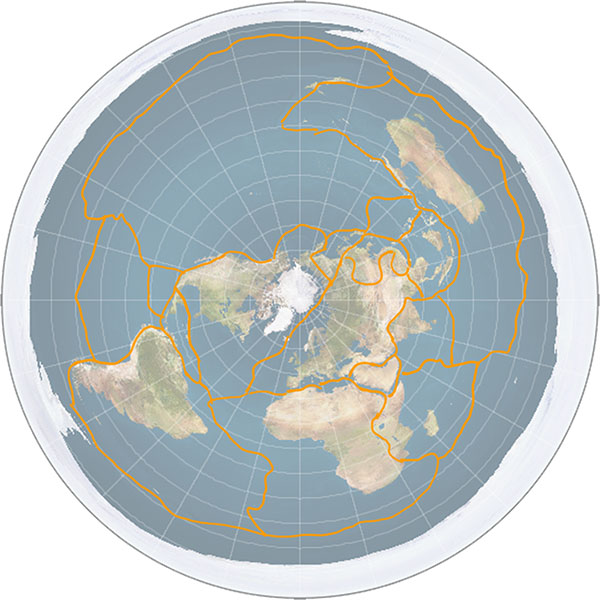
At least, the waves spread out in circles on a spherical Earth. In a flat Earth model, such as the typical “north pole in the middle” one, the spread of seismic waves produces elongated elliptical shapes or kidney shapes (such as the ones drawn in 23: Straight line travel), for no apparent or explicable reason.

P wave propagation times from Washington, flat Earth

Predicted P wave propagation time in minutes from an earthquake epicentre in Washington State, USA, projected onto a flat Earth.

P wave propagation times from Panama, flat Earth

Predicted P wave propagation time in minutes from an earthquake epicentre near Panama, projected onto a flat Earth.

P wave propagation times from Ecuador, flat Earth

Predicted P wave propagation time in minutes from an earthquake epicentre near Ecuador, projected onto a flat Earth.

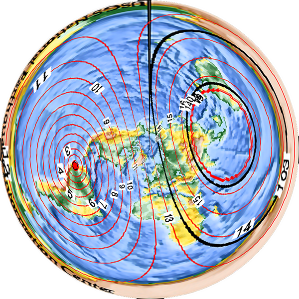
Why should seismic waves propagate more slowly towards or away from the North Pole, and faster along tangential arcs? Why would they take longer to reach an area in the middle of the opposing half of the disc than to reach the far edge of the disc, which is further away? There is no a priori reason, and any proposed justification is yet another ad hoc bandage on the model.

So the propagation speeds of the various seismic waves and the travel times to recording stations provide another proof that the Earth is a globe.

Note: There is more to be said about the propagation of seismic waves, which will provide another, different proof that the Earth is a globe. Some readers no doubt have a good idea what it is already. Rest assured that I haven’t overlooked it, and it will be covered in detail in a future article.

References:

[1] Athanasopoulos, G., Pelekis, P., Anagnostopoulos, G. A. “Effect of soil stiffness in the attenuation of Rayleigh-wave motions from field measurements”, Soil Dynamics and Earthquake Engineering, 19, p. 277-288, 2000. https://doi.org/10.1016/S0267-7261(00)00009-9

[2] Quang, P. B., Gaillard, P., Cano, Y. “Association of array processing and statistical modelling for seismic event monitoring”, Proceedings of the 23rd European Signal Processing Conference (EUSIPCO 2015), p. 1945-1949, 2015. https://doi.org/10.1109/EUSIPCO.2015.7362723

[3] International Seismological Centre (2020), International Seismograph Station Registry (IR). https://doi.org/10.31905/EL3FQQ40

34. Earth’s internal heat

Opening disclaimer: I’m going to be talking about “heat” a lot in this one. Formally, “heat” is defined as a process of energy flow, and not as an amount of thermal energy in a body. However to people who aren’t experts in thermodynamics (i.e. nearly everyone), “heat” is commonly understood as an “amount of hotness” or “amount of thermal energy”. To avoid the linguistic awkwardness of using the five-syllable phrase “thermal energy” in every single instance, I’m just going to use this colloquial meaning of “heat”. Even some of the papers I cite use “heat” in this colloquial sense. I’ve already done it in the title, which to be technically correct should be the more awkward and less pithy “Earth’s internal thermal energy”.

The interior of the Earth is hot. Miners know first hand that as you go deeper into the Earth, the temperature increases. The deepest mine on Earth is the TauTona gold mine in South Africa, reaching 3.9 kilometres below sea level. At this depth, the rock temperature is 60°C, and considerable cooling technology is required to bring the air temperature down to a level where the miners can survive. The Kola Superdeep Borehole in Russia reached a depth of 12.2 km, where it found the temperature to be 180°C.

Lava—molten rock—emerging from the Earth in Hawaii. (Public domain image by the United States Geological Survey, from Wikimedia Commons.)

Deeper in the Earth, the temperature gets hot enough to melt rock. The results are visible in the lava that emerges from volcanic eruptions. How did the interior of the Earth get that hot? And exactly how hot is it down there?

For many years, geologists have been measuring the amount of thermal energy flowing out of the Earth, at thousands of measuring stations across the planet. A 2013 paper analyses some 38,374 heat flow measurements across the globe to produce a map of the mean heat flow out of the Earth, shown below[1]:

Mean heat flow out of the Earth

Mean heat flow out of the Earth in milliwatts per square metre, as a function of location. (Figure reproduced from [1].)

From the map, you can see that most of Earth’s heat emerges at the mid-ocean ridges, deep underwater. This makes sense, as this is where rising plumes of magma from deep within the mantle are acting to bring new rock material to the crust. The coolest areas are generally geologically stable regions in the middle of tectonic plates.

Subterranean material (and heat) emerging from a hydrothermal vent on Eifuku Seamount, Marianas Trench Marine National Monument. (Public domain image by the United States National Oceanic and Atmospheric Administration, from Wikimedia Commons.)

Although the heat flow out of the Earth’s surface is of the order of milliwatts per square metre, the surface has a lot of square metres. The overall heat flow out of the Earth comes to a total of around 47 terawatts[2]. In contrast, the sun emits close to 4×10¹⁴ terawatts of energy in total, and the solar energy falling on the Earth’s surface is 1360 watts per square metre, over 10,000 times as much as the heat energy leaking out of the Earth itself. So the sun dominates Earth’s heating and weather systems by roughly that factor.

So the Earth generates some 47 TW of thermal power. Where does this huge amount of energy come from? To answer that, we need to go all the way back to when the Earth was formed, some 4.5 billion years ago.

Our sun formed from the gaseous and dusty material distributed throughout the Galaxy. This material is not distributed evenly, and where there is a denser concentration, gravity acts to draw in more material. As the material is pulled in, any small motions are amplified into an overall rotation. The result is an accretion disc, with matter spiralling into a growing mass at the centre. When the central concentration accumulates enough mass, the pressure ignites nuclear reactions and a star is born. Some of the leftover material continues to orbit the new star and forms smaller accretions that eventually become planets or smaller bodies.

The process of accreting matter generates thermal energy. Gravitational potential energy reduces as matter pulls closer together, and the resulting collisions between matter particles convert it into thermal energy, heating up the accumulating mass. Our Earth was born hot. As the matter settled into a solid body, the shrinking further heated the core through the Kelvin-Helmholtz mechanism. The total heat energy from the initial formation of the Earth dissipates only very slowly into space, and that process is still going on today, 4.5 billion years later.

It’s not known precisely how much of this primordial heat is left in Earth or how much flows out, but various different studies suggest it is somewhere in the range of 12-30 TW, roughly a quarter to two-thirds of Earth’s total measured heat flux[3]. So that’s not the only source of the heat energy flowing out of the Earth.

The other source of Earth’s internal heat is radioactive decay. Some of the matter in the primordial gas and dust cloud that formed the sun and planets was produced in the supernova explosions of previous generations of stars. These explosions produce atoms of radioactively unstable isotopes. Many of these decay relatively rapidly and are essentially gone by now. But some isotopes have very long half-lives, most importantly: potassium-40 (1.25 billion years), thorium-232 (14.05 billion years), uranium-235 (703.8 million years), and uranium-238 (4.47 billion years). These isotopes still exist in significant quantities inside the Earth, where they continue to decay, releasing energy.

We have a way of probing how much radioactive energy is released inside the Earth. The decay reactions produce neutrinos (which we’ve met before), and because they travel unhindered through the Earth these can be detected by neutrino observatories. These geoneutrinos have energy ranges that distinguish them from cosmic neutrino sources, and of course always emerge from underground. The observed decay rates from geoneutrinos correspond to a total radiothermal energy production of 10-30 TW, of the same order as the primordial heat flux. (The neutrinos themselves also carry away part of the energy from the radioactive decays, roughly 5 TW, but this is an additional component not deposited as thermal energy inside the Earth.)

Approximate radiothermal energy generated within the Earth, plotted as a function of time, from the formation of the Earth 4.5 billion years ago, to the present. The four main isotopes are plotted separately, and the total is shown as the dashed line. (Public domain figure adapted from data in [4], from Wikimedia Commons.)

To within the uncertainties, the sum of the estimated primordial and measured radiothermal energy fluxes is equal to the total measured 47 TW flux. So that’s good.

Once you know how much heat is being generated inside the Earth, you can start to apply heat transfer equations, knowing the thermodynamic properties of rock and iron, how much conduction and convection can be expected, and cross-referencing it with our knowledge of the physical state of these materials under different temperature and pressure conditions. There’s also additional information about the internal structure of the Earth that we get from seismology, but that’s a story for a future article. Putting it all together, you end up with a linked series of equations which you can solve to determine the temperature profile of the Earth as a function of depth.

Mean heat flow out of the Earth

Temperature profile of the Earth’s interior, from the surface (left) to the centre of the core (right). Temperature units are not marked on the vertical axis, but the temperature of the surface (bottom left corner) is approximately 300 K, and the inner core (IC, right) is around 7000 K. UM is upper mantle, LM lower mantle, OC outer core. The calculated temperature profile is the solid line. The two solid dots are fixed points constrained by known phase transitions of rock and iron – the slopes of the curves between them are governed by the thermodynamic equations. The dashed lines are various components of the constraining equations. (Figure reproduced from [5].)

The results are all self-consistent, with observations such as the temperature of the rock in deep mine shafts and the rate of detection of geoneutrinos, with structural constraints provided by seismology, and with the temperature constraints and known modes of heat flow from the core to the surface of the Earth.

That is, they’re all consistent assuming the Earth is a spherical body of rock and iron. If the Earth were flat, the thermal transport equations would need to be changed to reflect the different geometry. As a first approximation, assume the flat Earth is relatively thin (i.e. a cylinder with the radius larger than the height). We still measure the same amount of heat flux emerging from the Earth’s surface, so the same amount of heat has to be either (a) generated inside it, or (b) being input from some external energy source underneath the flat Earth. However geoneutrino energy ranges indicate that they come from radioactive decay of Earthly minerals, so it makes sense to conclude that radiothermal heating is significant.

If radioactive decay is producing heat within the bulk of the flat Earth, then half of the produced neutrinos will emerge from the underside, and thus be undetectable. So the total heat production should be double that deduced from neutrino observations, or somewhere in the range 20-60 TW. To produce twice the energy, you need twice the mass of the Earth. If the flat Earth is a disc with radius 20,000 km (the distance from the North Pole to the South Pole), then to have the same volume as the spherical Earth it would need to be 859 km thick. But we need twice as much mass to produce the observed thermal energy flux, so it should be approximately 1720 km thick. Some fraction of the geoneutrinos will escape from the sides of the cylinder of this thickness, which means we need to add more rock to produce a bit more energy to compensate, so the final result will be a bit thicker.

There’s no obvious reason to suppose that a flat Earth can’t be a bit over 1700 km thick, as opposed to any other thickness. With over twice as much mass as our spherical Earth, the surface gravity of this thermodynamically correct flat Earth would be over 2 Gs (i.e. twice the gravity we experience), which is obviously wrong, but then many flat Earth models deny Newton’s law of gravity anyway (because it causes so many problems for the model).

But just as in the spherical Earth model the observed geoneutrino flux only accounts for roughly half the observed surface heat flux. The other half could potentially come from primordial heat left over from the flat Earth’s formation – although as we’ve already seen, what we know about planetary formation precludes the formation of a flat Earth in the first place. The other option is (b) that the missing half of the energy is coming from some source underneath the flat Earth, heating it like a hotplate. What this source of extra energy is is mysterious. No flat Earth model that I’ve seen addresses this problem, let alone proposes a solution.

What’s more, if such a source of energy under the flat Earth existed, then it would most likely also radiate into space around the edges of the flat Earth, and have observable effects on the objects in the sky above us. What we’re left with, if we trust the sciences of radioactive decay and thermal energy transfer, is a strong constraint on the thickness of the flat Earth, plus a mysterious unspecified energy source underneath – neither of which are mentioned in standard flat Earth models.

References:

[1] Davies, J. H. “Global map of solid Earth surface heat flow”. Geochemistry, Geophysics, Geosystems, 14(10), p.4608-4622, 2013. https://doi.org/10.1002/ggge.20271

[2] Davies, J.H., Davies, D.R. “Earth’s surface heat flux”. Solid Earth, 1(1), p.5-24, 2010. https://doi.org/10.5194/se-1-5-2010

[3] Dye, S.T. “Geoneutrinos and the radioactive power of the Earth”. Reviews of Geophysics, 50(3), 2012. https://doi.org/10.1029/2012RG000400

[4] Arevalo Jr, R., McDonough, W.F., Luong, M. “The K/U ratio of the silicate Earth: Insights into mantle composition, structure and thermal evolution”. Earth and Planetary Science Letters, 278(3-4), p.361-369, 2009. https://doi.org/10.1016/j.epsl.2008.12.023

[5] Boehler, R. “Melting temperature of the Earth’s mantle and core: Earth’s thermal structure”. Annual Review of Earth and Planetary Sciences, 24(1), p.15-40, 1996. https://doi.org/10.1146/annurev.earth.24.1.15

22. Plate tectonics

Following the rediscovery of the New World by Europeans in the 15th century, the great seafaring nations of Europe rapidly mapped the eastern coastlines of the Americas. Demand for maps grew, not just of the New World, but of the Old as well. This made it possible for a young man (unfortunately women were shepherded into more domestic jobs) to seek his fortune as a mapmaker. One such man was Abraham Ortelius, who lived in Antwerp in the Duchy of Brabant (now part of Belgium).

Abraham Ortelius, painted by Peter Paul Rubens. (Public domain image from Wikimedia Commons.)

In 1547, at the age of 20, Ortelius began his career as a map engraver and illuminator. He travelled widely across Europe, and met cartographer and mapmaker Gerardus Mercator (15 years his senior, and whose map projection we met in 14. Map projections) in 1554. The two became friends and travelled together, reinforcing Ortelius’s passion for cartography, as well as the technical and scientific aspects of geography. Ortelius went on to produce and publish several maps of his own, culminating in his 1570 publication, Theatrum Orbis Terrarum (“Theatre of the Orb of the World”), now regarded as the first modern atlas of the world (as then known). Previously maps had been sold as individual sheets or bespoke sets customised to specific needs, but this was a curated collection intended to cover the entire known world in a consistent style. The Theatrum was wildly successful, running to 25 editions in seven languages by the time of Ortelius’s death in 1598.

World map plate from Theatrum Orbis Terrarum. (Public domain image from Wikimedia Commons.)

Being intimately familiar with his maps, Ortelius noticed a strange coincidence. In his publication Thesaurus Geographicus (“Geographical Treasury”) he wrote about the resemblance of the shapes of the east coast of the Americas to the west coasts of Europe and Africa across the Atlantic Ocean. He suggested that the Americas may have been “torn away from Europe and Africa … by earthquakes and floods. … The vestiges of the rupture reveal themselves, if someone brings forward a map of the world and considers carefully the coasts of the three.” This is the first known suggestion that the uncanny jigsaw-puzzle appearance of these coastlines might not be a coincidence, but rather a vestige of the continents actually having fitted together in the past.

Ortelius wasn’t the only one to make this observation and reach the same conclusion. Over the next few centuries, similar thoughts were proposed by geographers Theodor Christoph Lilienthal, Alexander von Humboldt, Antonio Snider-Pellegrini, Franklin Coxworthy, Roberto Mantovani, William Henry Pickering, Frank Bursley Taylor, and Eduard Suess. Suess even suggested (in 1885) that at some time in the past all of the Earth’s continents were joined in a single mass, which he gave the name “Gondwana”.

Illustration by Antonio Snider-Pellegrini, of his proposal that the Americas had once been adjacent to Europe and Africa. (Public domain image from Wikimedia Commons.)

Although many people had suggested that the continents had once been adjacent, nobody had produced any supporting evidence, nor any believable mechanism for how the continents could move. This changed in 1912, when the German meteorologist and polar scientist Alfred Wegener proposed the theory which he named continental drift. He began with the same observation of the jigsaw nature of the continent shapes, but then he applied the scientific method: he tested his hypothesis. He looked at the geology of coastal regions, examining the types of rocks, the geological structures, and the types of fossils found in places around the world. What he found were remarkable similarities in all of these features on opposite sides of the Atlantic Ocean, and in other locations around the world where he supposed that now-separate landmasses had once been in contact. This is exactly what you would expect to find if a long time ago the continents had been adjacent: plants and animals would have a range spanning across what would later split open and become an ocean, and geological features would be consistent across the divide as well[1].

Map of similar fossils of non-sea-going lifeforms found across landmasses, providing evidence that they were once joined. (Public domain image from Wikimedia Commons.)

In short, Wegener found and presented evidence in support of his hypothesis. He presented his theory, with the evidence he had gathered, in his 1915 book, Die Entstehung der Kontinente und Ozeane (“The Emergence of the Continents and Oceans”). He too proposed that all of the Earth’s continents were at one stage joined into a single landmass, which he named Pangaea (Greek for “all Earth”)[2].

But Wegener had two problems. Firstly, he still didn’t know how continents could possibly move. Secondly, he wasn’t a geologist, and so the establishment of geologists didn’t take him very seriously, to say the least. But as technology advanced, detailed measurements of the sea floor were made beginning in the late 1940s, including the structures, rock types, and importantly the magnetic properties of the rocks. Everything that mid-20th century geologists found was consistent with the existence of a large crack running down the middle of the Atlantic Ocean, where new rock material was welling up from beneath the ocean floor, and spreading outwards. They also found areas where the Earth’s crust was being squashed together, and either being thrust upwards like wrinkles in a tablecloth (such as the Himalayas mountain range), or plunged below the surface (such as along the west coast of the Americas).

Confronted with overwhelming evidence—which it should be pointed out was both consistent with many other observations, and also explained phenomena such as earthquakes and volcanoes better than older theories—the geological consensus quickly turned around[3]. The newly formulated theory of plate tectonics was as unstoppable as continental drift itself, and revolutionised our understanding of geology in the same way that evolution did for biology. Suddenly everything made sense.

The Earth, we now know, has a relatively thin, solid crust of rocks making up the continents and sea floors. Underneath this thin layer is a thick layer known as the mantle. The uppermost region of the mantle is solid and together with the crust forms what is known as the lithosphere. Below this region, most of the mantle is hot enough that the material there is visco-elastic, meaning it behaves like a thick goopy fluid, deforming and flowing under pressure. This viscous region of the mantle is known as the asthenosphere.

Diagram of the Earth’s layers. The lithosphere region is not to scale and would appear much thinner if drawn to scale. (Public domain image from Wikimedia Commons.)

Heat wells up from the more central regions of the Earth (generated by radioactive decay). Just like a boiling pot of water, this sets up convection currents in the asthenosphere, where the hot material flows upward, then sideways, then back down to form a loop. The sideways motion at the top of these convection cells is what carries the crust above, moving it slowly across the surface of the planet.

The Earth’s crust is broken into pieces, called tectonic plates, which fit together along their edges. Each plate is relatively rigid, but moves relative to the other plates. Plates move apart where the upwelling of the convection cells occurs, such as along the Mid-Atlantic Ridge (the previously mentioned crack in the Atlantic Ocean floor), and collide and subduct back down along other edges. At some plate boundaries the plates slide horizontally past one another. All of this motion causes earthquakes and volcanoes, which are mostly concentrated along the plate boundaries. The motion of the plates is slow, around 10-100 millimetres a year. This is too slow to notice over human history, except with high-tech equipment. GPS navigation and laser ranging systems can directly measure the movements of the continents relative to one another, confirming the speed of the motion.

The tectonic plates, then, are shell-like pieces of crust that fit together to form the spherical shape of the Earth’s surface. An equal amount of area is lost at subduction zones as is gained by spreading on sea-floors and in places such as Africa’s Rift Valley, keeping the Earth’s surface area constant. As the plates drift around, they don’t change in size or deform geometrically very much.

Earth's tectonic plates

Sketch of the major tectonic plates as they fit together to form the surface of the Earth.

All of this is consistent and supported by many independent pieces of evidence. Direct measurement shows that the continents are moving, so it’s really just a matter of explaining how. But the motions of the tectonic pates only make sense on a globe.

If the Earth were flat, then sure, you could conceivably have some sort of underlying structure that supports the same sort of convection cells and geological processes of spreading and subduction, leading to earthquakes and volcanoes, and so on. But look at the shapes of the tectonic plates.

Earth's tectonic plates on a flat Earth

Sketch of the major tectonic plates on a flat Earth.

Because of the distortions in the shape of the map relative to a globe, the tectonic plates need to change shape and size as they move across the surface. Not only that, but consider the Antarctic plate, which is a perfectly normal plate on the globe. On the typical Flat Earth model where Antarctica is a barrier of ice around the edge of the circle, the Antarctic plate is a ring. And when it moves, it not only has to deform in shape, but crust has to disappear off one side of the disc and appear on the other side.

So plate tectonics, the single most fundamental and important discovery in the entire field of geology, only makes sense because the Earth is a globe.

Notes:

[1] For readers interested in this particular aspect of continental drift, I’ve previously written about it at greater length in the annotation to this Irregular Webcomic! http://www.irregularwebcomic.net/1946.html

[2] Pangaea is now the accepted scientific term for the unified landmass when all the continents were joined. Eduard Suess’s Gondwana lives on as the name now used to refer to the conjoined southern continents before merging with the northern ones to form Pangaea.

[3] Alfred Wegener is often cited by various people in support of the idea that established science often laughs at revolutionary ideas proposed by outsiders, only for the outsider to later be vindicated. Often by people proposing outlandish or fringe science theories that defy not only scientific consensus but also the boundaries of logic and reason. What they fail to point out is that in all the history of science, Wegener is almost the only such case, whereas almost every other outsider proposing a radical theory is shown to be wrong. As Carl Sagan so eloquently put it in Broca’s Brain:

The fact that some geniuses were laughed at does not imply that all who are laughed at are geniuses. They laughed at Columbus, they laughed at Fulton, they laughed at the Wright brothers. But they also laughed at Bozo the Clown.

Share this:

Share this:

Share this: