41. Cosmic rays

The French physicist Henri Becquerel discovered the phenomenon of radioactivity in 1896, while performing experiments on phosphorescence – the unrelated phenomenon that causes “glow in the dark” materials to glow for several minutes after being exposed to light. He was interested to see if phosphorescence was related to x-rays, discovered only a few months earlier by Wilhelm Roentgen. In his experiments, Becquerel noticed that uranium salts could darken photographic film, even if wrapped in black paper so that no light could fall on the film, and even from non-phosphorescent uranium samples. The conclusion was that some sort of penetrating rays were being emitted by the uranium itself, without being excited by external energy.

Henri Becquerel in his lab width=

Henri Becquerel in his lab. (Public domain image from Wikimedia Commons.)

Marie and Pierre Curie quickly discovered other radioactive elements, and Becquerel himself discovered by experimenting with magnets that there were three different types of radioactive radiation: two deflected in different directions by a magnetic field and one not deflected at all. In 1899, Ernest Rutherford characterised the first two types, naming them alpha and beta particles, with positive and negative electric charges. Becquerel measured the mass/charge ratio of beta particles in 1900 and determined that they were the same as the electrons discovered by J. J. Thomson in 1897. In 1907 Rutherford showed that alpha particles were the nuclei of helium atoms. And in 1914, he showed that the third type of radiation, named gamma rays, were a form of electromagnetic radiation.

Ernest Rutherford with Hans Geiger

Ernest Rutherford (right), in his lab with Hans Geiger (left), inventor of the Geiger counter. (Public domain image from Wikimedia Commons.)

This was an exciting time in physics, and our understanding of atomic structure was revolutionised within the space of two decades. Besides discovering the basic structure of the atom and how it related to the phenomenon of radioactive decay, several peripheral phenomena also came to the attention of scientists.

One observation was that atoms in the atmosphere were sometimes ionised, or “electrified” as the scientists of the time described it. Ionisation is the process of electrons being stripped off neutral atoms, to form negatively charged free electrons and positively charged atomic ions (consisting of the atomic nucleus and a less-than-full complement of electrons). It was clear that radioactive rays could ionise atoms in the air, and so scientists assumed that it was radiation from radioactive elements in the ground that was ionising the air near ground level.

Father Theodor Wulf

Except strangely the amount of ionising radiation in the atmosphere seemed to increase with increasing altitude. German physicist and Jesuit priest Theodor Wulf invented in 1909 a portable electroscope capable of measuring the ionisation of the atmosphere. He used it to investigate the source of the ionising radiation by measuring ionisation at the base and the top of the Eiffel Tower. He found that the ionisation at the top of the 300 metre tower was a bit over half that at ground level, which was higher than he expected, since theoretically he expected the ionisation to drop by half every 80 metres, so to be less than one tenth the ionisation at ground level. He concluded that there must be some other source of ionising radiation coming from above the atmosphere. However, his published paper was largely ignored.

In 1911, the Italian physicist Domenico Pacini measured the ionisation rates in various places, including mountains, lakes, seas, and underwater. He showed that the rate dropped significantly underwater, and concluded that the main source of radiation could not be the Earth itself. Then in 1912, Austrian physicist Victor Hess took some Wulf electroscopes up in a hot air balloon to altitudes as high as 5300 metres, flying both in daylight, night time, and during an almost complete solar eclipse.

Victor Hess in a hot air balloon flight

Victor Hess (centre), after one of his balloon flight experiments. (Public domain image from Wikimedia Commons.)

Hess showed that the amount of ionising radiation decreased as one moved from ground level up to about 1000 metres, but then increased again rapidly. At 5300 metres, there was approximately twice as much ionising radiation as at ground level.[1] And because the effect occurred at night, and during a solar eclipse, it wasn’t due to the sun. Hess had proven that there was a source of this radiation outside the Earth’s atmosphere. Further unmanned balloon flights as high as 9 km showed the radiation increased even higher with altitude.

Atmospheric radiation readings recorded by Victor Hess

Readings of ionising radiation level (columns 2 to 4) at different altitudes (column 1, in metres), as recorded by Victor Hess. (Figure reproduced from [1].)

What this mysterious radiation was remained unknown until the late 1920s. It was initially thought to be electromagnetic radiation (i.e. gamma rays and x-rays). Robert Millikan named them cosmic rays in 1925 after proving that they originated outside the Earth. Then in 1927 the Dutch physicist Jacob Clay performed measurements while sailing from Java to the Netherlands, which showed that their intensity increased as one moved from the tropics to mid-latitudes.[2] He correctly deduced that the intensity was affected by the Earth’s magnetic field, which implied the cosmic rays must be charged particles.

Atmospheric radiation readings recorded by Jacob Clay

Data recorded by Jacob Clay showing change in ionising radiation with latitude during his voyage from Java to Europe. (Figure reproduced from [2].)

In 1930, the Italian Bruno Rossi realised that if cosmic rays are electrically charged, then they should be deflected either east or west by the Earth’s magnetic field, depending on whether they are positively or negatively charged, respectively.[3] Experiments found that at all locations on the Earth’s surface there are more cosmic rays coming from the west than from the east, showing that most (if not all) cosmic ray particles are positively charged. This observation was called the east-west effect.

Illustration showing incoming cosmic rays deflected to the east

Illustration of the east-west effect. In the space around the Earth (shown as black in this diagram), the Earth’s magnetic field is directed perpendicularly out of the diagram. Incoming cosmic rays are shown in red. When they encounter Earth’s magnetic field, charged particles are deflected perpendicular to the field direction. Positively charged particles are deflected to the right, as shown, meaning that from the surface of the Earth, cosmic rays tend to preferentially come from the west.

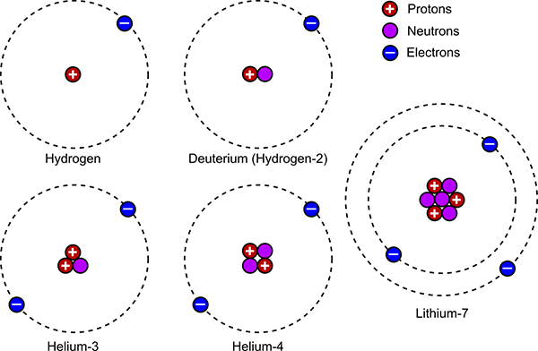
Subsequent experiments determined that around 90% of cosmic rays entering our atmosphere are protons, 9% are helium nuclei (or alpha particles), and the remaining 1% are nuclei of heavier elements, with an extremely small number of other types of particles. And in 1936, for his crucial part in the discovery in cosmic rays, Victor Hess was awarded the Nobel Prize for Physics.

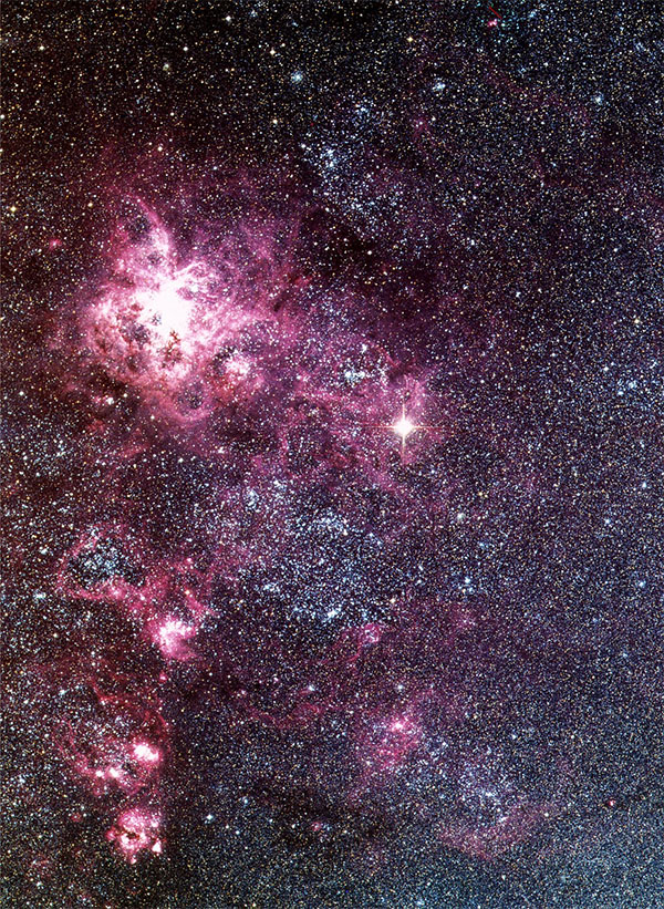
The origin of cosmic rays is however still not entirely clear. Our sun produces energetic particles that reach Earth, but cosmic rays are generally defined as coming from outside our own solar system. Our Milky Way Galaxy produces some of the lower energy particles, mostly from the direction of the galactic core, however at very high energies there is a deficit of cosmic rays in that direction, implying a shadowing effect on rays whose origin lies outside our galaxy. Known sources of cosmic rays include supernova explosions, supernova remnants (such as the Crab Nebula), active galactic nuclei, and quasars. But there are some very high energy cosmic rays whose source is still a mystery.

The fact that high energy cosmic rays originate from outside our galaxy, means that they should be isotropic – uniform in intensity distribution, independent of the direction from which they approach Earth. However, the Earth is not a stationary observation platform. The Earth orbits the sun at a speed of almost 30 km/s. But on a galactic scale this motion is dwarfed by the sun’s orbital speed around the core of our galaxy, which is 230 km/s, roughly in the direction of the star Vega, in the constellation Lyra. So relative to extragalactic cosmic rays, Earth is moving at an average speed of approximately 230 km/s. This speed adds to the energy of cosmic rays coming from the direction of Vega, and subtracts from the energies of cosmic rays coming from the opposite direction.

Diagram showing our sun's orbit about the galaxy

Our sun orbits the centre of the Milky Way Galaxy, at a speed of 230 km/s. This speed modifies the speed and direction of incoming cosmic rays from outside the Galaxy. (Modified from a public domain image by NASA, from Wikimedia Commons.)

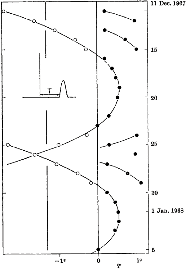
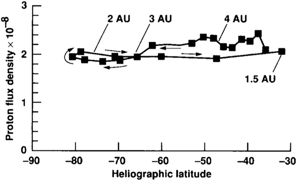
This difference is known as the Compton-Getting effect after the discoverers Arthur Compton and Ivan Getting.[4] It produces about a 0.1% difference in the energies of cosmic rays coming from the opposite directions, which can be observed statistically. The effect was confirmed experimentally in 1986.[5]

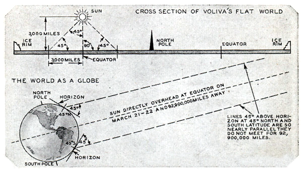
So we have two different observational effects that have been experimentally confirmed in the distribution of cosmic rays arriving at Earth. The Compton-Getting effect shows that the Earth is moving in the direction of the star Vega. Vega is of course above the Earth’s horizon as seen from half the planet’s surface at any one time, and below the horizon (behind the planet) from the other half of the Earth’s surface. By measuring cosmic ray distributions, you can show that the direction defined by the Compton-Getting anisotropy relative to the ground plane varies depending on your position on Earth. In other words, by measuring cosmic rays, you can prove that the Earth’s direction of motion through the galaxy is upwards from the ground in one place, while simultaneously downwards into the ground from a point on the opposite side of the planet, and at intermediate angles in places in between. Which is perfectly consistent for a spherical planet, but inconsistent with a Flat Earth.

The second effect, the east-west effect, is also readily explained with a spherical Earth, with the addition of a simple dipole magnetic field. As can be seen in the diagram above (“Illustration of the east-west effect”), incoming positively charged cosmic rays are uniformly deflected to the right (as viewed from above Earth’s North Pole), resulting in more rays arriving from the west than from the east, independent of location or time of day. The same observed east-west effect could in theory be produced on a Flat Earth, but only if the magnetic field is flattened out as well, holding the same relative orientation to the Earth’s surface as it does on the globe.

Magnetic field as required for the east-west effect, on spherical and flat Earths

Shape of magnetic fields to produce the observed east-west effect in incoming cosmic rays. The required magnetic field for a spherical Earth is very close to a simple dipole, easily generated with known physical principles. The required magnetic field shape for a flat Earth is severely flattened, and cannot be produced with a simple magnetic dynamo model.

This would result in the field being grossly distorted from that of a simple dipole, and thus requiring some exotic method of generating such a complex field – a complex field that just happens to mimic exactly the field of a straightforward dipole if the Earth were spherical. In another application of Occam’s razor (similar to its use in article 8. Earth’s magnetic field), it is more parsimonious to conclude that the Earth is not flat, but spherical.

References:

[1] Hess, V.F. “Über Beobachtungen der durchdringenden Strahlung bei sieben Freiballonfahrten” (Observation of penetrating radiation in seven free balloon flights). Physikalische Zeitschrift, 13, p.1084-1091, 1912. http://inspirehep.net/record/1623161/

[2] Clay, J. “Penetrating radiation”. Proceedings of the Royal Academy of Sciences Amsterdam, 30, p. 1115-1127, 1927. https://www.dwc.knaw.nl/DL/publications/PU00011919.pdf

[3] Rossi, B. “On the magnetic deflection of cosmic rays”. Physical Review, 36(3), p. 606, 1930. https://doi.org/10.1103/PhysRev.36.606

[4] Compton, A. H., Getting, I. A. “An Apparent Effect of Galactic Rotation on the Intensity of Cosmic Rays”. Physical Review, 47, p. 817-821, 1935. https://doi.org/10.1103/PhysRev.47.817

[5] Cutler, D., Groom, D. “Observation of terrestrial orbital motion using the cosmic-ray Compton–Getting effect”. Nature, 322, p. 434-436, 1986. https://doi.org/10.1038/322434a0

30. Pulsar timing

In our last entry on neutrino beams, we met James Chadwick, who discovered the existence of the neutron in 1932. The neutron explained radioactive beta decay as a process in which a neutron decays into a proton, an electron, and an electron antineutrino. This also means that a reverse process, known as electron capture, is possible: a proton and an electron may combine to form a neutron and an electron neutrino. This is sometimes also known as inverse beta decay, and occurs naturally for some isotopes with a relative paucity of neutrons in the nucleus.

Electron capture

Electron capture. A proton and electron combine to form a neutron. An electron neutrino is emitted in the process.

In most circumstances though, an electron will not approach a proton close enough to combine into a neutron, because there is a quantum mechanical energy barrier between them. The electron is attracted to the proton by electromagnetic force, but if it gets too close then its position becomes increasingly localised and by Heisenberg’s uncertainty principle its energy goes up correspondingly. The minimum energy state is the orbital distance where the electron’s probability distribution is highest. In electron capture, the weak nuclear force overcomes this energy barrier.

Electron capture energy diagram

Diagram of electron energy at different distances from a proton. Far away, electrostatic attraction pulls the electron closer, but if it gets too close, Heisenberg uncertainty makes the kinetic energy too large, so the electron settles around the minimum energy distance.

But you can also overcome the energy barrier by providing external energy in the form of pressure. Squeeze the electron and proton enough and you can push through the energy barrier, forcing them to combine into a neutron. In 1934 (less than 2 years after Chadwick discovered the neutron), astronomers Walter Baade and Fritz Zwicky proposed that this could happen naturally, in the cores of large stars following a supernova explosion (previously discussed in the article on supernova 1987A).

During a star’s lifetime, the enormous mass of the star is prevented from collapsing under its own gravity by the energy produced by nuclear fusion in the core. When the star begins to run out of nuclear fuel, that energy is no longer sufficient to prevent further gravitational collapse. Small stars collapse to a state known as a white dwarf, in which the minimal energy configuration has the atoms packed closely together, with electrons filling all available quantum energy states, so it’s not possible to compress the matter further. However, if the star has a mass greater than about 1.4 times the mass of our own sun, then the resulting pressure is so great that it overwhelms the nuclear energy barrier and forces the electrons to combine with protons, forming neutrons. The star collapses even further, until it is essentially a giant ball of neutrons, packed shoulder to shoulder.

These collapses, to a white dwarf or a so-called neutron star, are accompanied by a huge and sudden release of gravitational potential energy, which blows the outer layers of the star off in a tremendously violent explosion, which is what we can observe as a supernova. Baade and Zwicky proposed the existence of neutron stars based on the understanding of physics at the time. However, they could not imagine any method of ever detecting a neutron star. A neutron star would, they imagined, simply be a ball of dead neutrons in space. Calculations showed that a neutron star would have a radius of about 10 kilometres, making them amazingly dense, but correspondingly difficult to detect at interstellar distances. So neutron stars remained nothing but a theoretical possibility for decades.

In July 1967, Ph.D. astronomy student Jocelyn Bell was observing with the Interplanetary Scintillation Array at the Mullard Radio Astronomy Observatory in Cambridge, under the tutelage of her supervisor Antony Hewish. She was looking for quasars – powerful extragalactic radio sources which had recently been discovered using the new observation technique of radio astronomy. As the telescope direction passed through one particular patch of sky in the constellation of Vulpecula, Bell found some strange radio noise. Bell and Hewish had no idea what the signal was. At first they assumed it must be interference from some terrestrial or known spacecraft radio source, but over the next few days Bell noticed the signal appearing 4 minutes earlier each day. It was rising and setting with the stars, not in synch with anything on Earth. The signal was from outside our solar system.

Bell suggested running the radio signal strength plotter at faster speeds to try to catch more details of the signal. It took several months of persistent work, examining kilometres of paper plots. Hewish considered it a waste of time, but Bell persisted, until in November she saw the signal drawn on paper moving extremely rapidly through the plotter. The extraterrestrial radio source was producing extremely regular pulses, about 1 1/3 seconds apart.

PSR B1919+21 trace

The original chart recorder trace containing the detection signal of radio pulses from the celestial coordinate right ascension 1919. The pulses are the regularly spaced downward deflections in the irregular line near the top. (Reproduced from [1].)

This was exciting! Bell and Hewish thought that it might possibly be a signal produced by alien life, but they wanted to test all possible natural sources before making any sort of announcement. Bell soon found another regularly pulsating radio source in a different part of the sky, which convinced them that it was probably a natural phenomenon.

They published their observations[2], speculating that the pulses might be caused by radial oscillation in either white dwarfs or neutron stars. Fellow astronomers Thomas Gold and Fred Hoyle, however, immediately recognised that the pulses could be produced by the rotation of a neutron star.

Stars spin, relatively leisurely, due to the angular momentum in the original clouds of gas from which they formed. Our own sun rotates approximately once every 24 days. During a supernova explosion, as the core of the star collapses to a white dwarf or neutron star, the moment of inertia reduces in size and the rotation rate must increase correspondingly to conserve angular momentum, in the same way that a spinning ice skater speeds up by pulling their arms inward. Collapsing from stellar size down to 10 kilometres produces an increase in rotation rate from once per several days to the incredible rate of about once per second. At the same time, the star’s magnetic field is pulled inward, greatly strengthening it. Far from being a dead ball of neutrons, a neutron star is rotating rapidly, and has one of the strongest magnetic fields in nature. And when a magnetic field oscillates, it produces electromagnetic radiation, in this case radio waves.

The magnetic poles of a neutron star are unlikely to line up exactly with the rotational axis. Radio waves are generated by the rotation and funnelled out along the magnetic poles, forming beams of radiation. So as the neutron star rotates, these radio beams sweep out in rotating circles, like lighthouse beacons. A detector in the path of a radio beam will see it flash briefly once per rotation, at regular intervals of the order of one second – exactly what Bell observed.

Pulsar diagram

Diagram of a pulsar. The neutron star at centre has a strong magnetic field, represented by field lines in blue. I the star rotates about a vertical axis, the magnetic field generates radio waves beamed in the directions shown by the purple areas, sweeping through space like lighthouse beacons. (Public domain image by NASA, from Wikimedia Commons.)

Radio-detectable neutron stars quickly became known as pulsars, and hundreds more were soon detected. For the discovery of pulsars, Antony Hewish was awarded the Nobel Prize in Physics in 1974, however Jocelyn Bell (now Jocelyn Bell Burnell after marriage) was overlooked, in what has become one of the most notoriously controversial decisions ever made by the Nobel committee.

Jocelyn Bell Building

Image of Jocelyn Bell Burnell on the Jocelyn Bell Building in the Parque Tecnológico de Álava, Araba, Spain. (Public domain image from Wikimedia Commons.)

Astronomers found pulsars in the middle of the Crab Nebula supernova remnant (recorded as a supernova by Chinese astronomers in 1054), the Vela supernova remnant, and several others, cementing the relationship between supernova explosions and the formation of neutron stars. Popular culture even got in on the act, with Joy Division’s iconic 1979 debut album cover for Unknown Pleasures featuring pulse traces from pulsar B1919+21, the very pulsar that Bell first detected.

By now, the strongest and most obvious pulsars have been discovered. To discover new pulsars, astronomers engage in pulsar surveys. A radio telescope is pointed at a patch of sky and the strength of radio signals received is recorded over time. The radio trace is noisy and often the pulsar signal is weaker than the noise, so it’s not immediately visible like B1919+21. To detect it, one method is to perform a Fourier transform on the signal, to look for a consistent signal at a specific repetition period. Unfortunately, this only works for relatively strong pulsars, as weak ones are still lost in the noise.

A more sensitive method is called epoch folding, which is performed by cutting the signal trace into pieces of equal time length and summing them all up. The noise, being random, tends to cancel out, but if a periodic signal is present at the same period as the sliced time length then it will stack on top of itself and become more prominent. Of course, if you don’t know the period of a pulsar present in the signal, you need to try doing this for a large range of possible periods, until you find it.

To further increase the sensitivity, you can add in signals recorded at different radio frequencies as well – most radio telescopes can record signals at multiple frequencies at once. A complication is that the thin ionised gas of the interstellar medium slows down the propagation of radio waves slightly, and it slows them down by different amounts depending on the frequency. So as the radio waves propagate through space, the different frequencies slowly drift out of synch with one another, a phenomenon known as dispersion. The total amount of dispersion depends in a known way on the amount of plasma travelled through—known as the dispersion measure—so measuring the dispersion of a pulsar gives you an estimate of how far away it is. The estimate is a bit rough, because the interstellar medium is not uniform – denser regions slow down the waves more and produce greater dispersion.

Pulsar dispersion

Dispersion of pulsar pulses. Each row is a folded and summed pulse profile over many observation periods, as seen at a different radio frequency. Note how the time position of the pulse drifts as the frequency varies. If you summed these up without correction for this dispersion, the signal would disappear. The bottom trace shows the summed signal after correction for the dispersion by shifting all the pulses to match phase. (Reproduced from [3].)

So to find a weak pulsar of unknown period and dispersion measure, you fold all the signals at some speculative period, then shift the frequencies by a speculative dispersion measure and add them together. Now we have a two-dimensional search space to go through. This approach takes a lot of computer time, trying many different time folding periods and dispersion measures, and has been farmed out as part of distributed “home science” computing projects. The pulsar J2007+2722 was the first pulsar to be discovered by a distributed home computing project[4].

But wait – there’s one more complication. The observed period of a pulsar is equal to the emission period if you observe it from a position in space that is not moving relative to the pulsar. If the observer is moving with respect to the pulsar, then the period experiences a Doppler shift. Imagine you are moving away from a pulsar that is pulsing exactly once per second. A first pulse arrives, but in the second that it takes the next pulse to arrive, you have moved further away, so the radio signal has to travel further, and it arrives a fraction of a second more than one second after the previous pulse. The difference is fairly small, but noticeable if you are moving fast enough.

The Earth moves around the sun at an orbital speed of 29.8 km/s. So if it were moving directly away from a pulsar, dividing this by the speed of light, each successive pulse would arrive 0.1 milliseconds later than if the Earth were stationary. This would actually not be a problem, because instead of folding at a period of 1.0000 seconds, we could detect the pulsar by folding at a period of 1.0001 seconds. But the Earth doesn’t move in a straight line – it orbits the sun in an almost circular ellipse. On one side of the orbit the pulsar period is measured to be 1.0001 s, but six months later it appears to be 0.999 s.

This doesn’t sound like much, but if you observe a pulsar for an hour, that’s 3600 seconds, and the cumulative error becomes 0.36 seconds, which is far more than enough to completely ruin your signal, smearing it out so that it becomes undetectable. Hewish and Bell, in their original pulsar detection paper, used the fact that they observed this timing drift consistent with Earth’s orbital velocity to narrow down the direction that the pulsar must lie in (their telescope received signals from a wide-ish area of sky, making pinpointing the direction difficult).

Timing drift of pulsar B1919+21

Timing drift of pulsar B1919+21 from Hewish and Bell’s discovery paper. Cumulative period timing difference on the horizontal axis versus date on the vertical axis. If the Earth were not moving through space, all the detection periods for different dates would line up on the 0. With no other data at all, you can use this graph to work out the period of Earth’s orbit. (Figure reproduced from [2].)

What’s more, not just the orbit of the Earth, but also the rotation of the Earth affects the arrival times of pulses. When a pulsar is overhead, it is 6370 km (the radius of the Earth) closer than when it is on the horizon. Light takes over 20 milliseconds to travel that extra distance – a huge amount to consider when folding pulsar data. So if you observe a pulsar over a single six-hour session, the period can drift by more than 0.02 seconds due to the rotation of the Earth.

These timing drifts can be corrected in a straightforward manner, using the astronomical coordinates of the pulsar, the latitude and longitude of the observatory, and a bit of trigonometry. So in practice these are the steps to detect undiscovered pulsars:

  1. Observe a patch of sky at multiple radio frequencies for several hours, or even several days, to collect enough data.
  2. Correct the timing of all the data based on the astronomical coordinates, the latitude and longitude of the observatory, and the rotation and orbit of the Earth. This is a non-linear correction that stretches and compresses different parts of the observation timeline, to make it linear in the pulsar reference frame.
  3. Perform epoch folding with different values of period and dispersion measure, and look for the emergence of a significant signal above the noise.
  4. Confirm the result by observing with another observatory and folding at the same period and dispersion measure.

This method has been wildly successful, and as of September 2019 there are 2796 known pulsars[5].

If step 2 above were omitted, then pulsars would not be detected. The timing drifts caused by the Earth’s orbit and rotation would smear the integrated signal out rather than reinforcing it, resulting in it being undetectable. The latitude and longitude of the observatory are needed to ensure the timing correction calculations are done correctly, depending on where on Earth the observatory is located. It goes almost without saying that the astronomers use a spherical Earth model to get these corrections right. If they used a flat Earth model, the method would not work at all, and we would not have detected nearly as many pulsars as we have.

Addendum: Pulsars are dear to my own heart, because I wrote my physics undergraduate honours degree essay on the topic of pulsars, and I spent a summer break before beginning my Ph.D. doing a student project at the Australia Telescope National Facility, taking part in a pulsar detection survey at the Parkes Observatory Radio Telescope, and writing code to perform epoch folding searches.

Some of the data I worked on included observations of pulsar B0540-69, which was first detected in x-rays by the Einstein Observatory in 1984[6], and then at optical wavelengths in 1985[7], flashing with a period of 0.0505697 seconds. I made observations and performed the data processing that led to the first radio detection of this pulsar[8]. (I’m credited as an author on the paper under my unmarried name.) I can personally guarantee you that I used timing corrections based on a spherical model of the Earth, and if the Earth were flat I would not have this publication to my name.

References:

[1] Lyne, A. G., Smith, F. G. Pulsar Astronomy. Cambridge University Press, Cambridge, 1990.

[2] Hewish, A., Bell, S. J., Pilkington, J. D. H., Scott, P. F., Collins, R. A. “Observation of a Rapidly Pulsating Radio Source”. Nature, 217, p. 709-713, 1968. https://doi.org/10.1038/217709a0

[3] Lorimer, D. R., Kramer, M. Handbook of Pulsar Astronomy. Cambridge University Press, Cambridge, 2012.

[4 Allen, B., Knispel, B., Cordes, J.; et al. “The Einstein@Home Search for Radio Pulsars and PSR J2007+2722 Discovery”. The Astrophysical Journal, 773 (2), p. 91-122, 2013. https://doi.org/10.1088/0004-637X/773/2/91

[5] Hobbs, G., Manchester, R. N., Toomey, L. “ATNF Pulsar Catalogue v1.61”. Australia Telescope National Facility, 2019. https://www.atnf.csiro.au/people/pulsar/psrcat/ (accessed 2019-10-09).

[6] Seward, F. D., Harnden, F. R., Helfand, D. J. “Discovery of a 50 millisecond pulsar in the Large Magellanic Cloud”. The Astrophysical Journal, 287, p. L19-L22, 1984. https://doi.org/10.1086/184388

[7] Middleditch, J., Pennypacker, C. “Optical pulsations in the Large Magellanic Cloud remnant 0540–69.3”. Nature. 313 (6004). p. 659, 1985. https://doi.org/10.1038/313659a0

[8] Manchester, R. N., Mar, D. P., Lyne, A. G., Kaspi, V. M., Johnston, S. “Radio Detection of PSR B0540-69”. The Astrophysical Journal, 403, p. L29-L31, 1993. https://doi.org/10.1086/186714

25. Planetary formation

Why does Earth exist at all?

The best scientific model we have for understanding how the Earth exists begins with the Big Bang, the event that created space and time as we know and understand it, around 14 billion years ago. Scientists are interested in the questions of what possibly happened before the Big Bang and what caused the Big Bang to happen, but haven’t yet converged on any single best model for those. However, the Big Bang itself is well established by multiple independent lines of evidence and fairly uncontroversial.

The very early universe was a hot, dense place. Less than a second after the Big Bang, it was essentially a soup of primordial matter and energy. The energy density was so high that the equivalence of mass and energy (discovered by Albert Einstein) allowed energy to convert into particle/antiparticle pairs and vice versa. The earliest particles we know of were quarks, electrons, positrons, and neutrinos. The high energy density also pushed space apart, causing it to expand rapidly. As space expanded, the energy density reduced. The particles and antiparticles annihilated, converting back to energy, and this process left behind a relatively small residue of particles.

Diagram of the Big Bang

Schematic diagram of the evolution of the universe following the Big Bang. (Public domain image by NASA.)

After about one millionth of a second, the quarks no longer had enough energy to stay separated, and bound together to form the protons and neutrons more familiar to us. The universe was now a plasma of charged particles, interacting strongly with the energy in the form of photons.

After a few minutes, the strong nuclear force could compete with the ambient energy level, and free neutrons bonded together with protons to form a few different types of atomic nuclei, in a process known as nucleosynthesis. A single proton and neutron could pair up to form a deuterium nucleus (an isotope of hydrogen, also known as hydrogen-2). More rarely, two protons and a neutron could combine to make a helium-3 nucleus. More rarely still, three protons and four neutrons occasionally joined to form a lithium-7 nucleus. Importantly, if two deuterium nuclei collided, they could stick together to form a helium-4 nucleus, the most common isotope of helium. The helium-4 nucleus (or alpha particle as it is also known in nuclear physics) is very stable, so the longer this process went on, the more helium nuclei were formed and the more depleted the supply of deuterium became. Ever since the Big Bang, natural processes have destroyed more of the deuterium, but created only insignificant additional amounts – which means that virtually all of the deuterium now in existence was created during the immediate aftermath of the Big Bang. This is important because measuring the abundance of deuterium in our universe now gives us valuable evidence on how long this phase of Big Bang nucleosynthesis lasted. Furthermore, measuring the relative abundances of helium-3 and lithium-7 also give us other constraints on the physics of the Big Bang. This is one method we have of knowing what the physical conditions during the very early universe must have been like.

Nuclei formed during the Big Bang

Diagrams of the nuclei (and subsequent atoms) formed during Big Bang nucleosynthesis.

The numbers all point to this nucleosynthesis phase lasting approximately 380,000 years. All the neutrons had been bound into nuclei, but the vast majority of protons were left bare. At this time, something very important happened. The energy level had lowered enough for the electrostatic attraction of protons and electrons to form the first atoms. Prior to this, any atoms formed would quickly be ionised again by the surrounding energy. The bare protons attracted an electron each and become atoms of hydrogen. The deuterium nuclei also captured an electron to become atoms of deuterium. The helium-3 and helium-4 nuclei captured two electrons each, while the lithium nuclei attracted three. There were two other types of atoms almost certainly formed which I haven’t mentioned yet: hydrogen-3 (or tritium) and beryllium-7 – however both of these are radioactive and have short half-lives (12 years for tritium; 53 days for beryllium-7), so within a few hundred years there would be virtually none of either left. And that was it – the universe had its initial supply of atoms. There were no other elements yet.

When the electrically charged electrons became attached to the charged nuclei, the electric charges cancelled out, and the universe changed from a charged plasma to an electrically neutral gas. This made a huge difference, because photons interact strongly with electrically charged particles, but much less so with neutral ones. Suddenly, the universe went from opaque to largely transparent, and light could propagate through space. When we look deep into space with our telescopes, we look back in time because of the finite speed of light (light arriving at Earth from a billion light years away left its source a billion years ago). This is the earliest possible time we can see. The temperature of the universe at this time was close to 3000 kelvins, and the radiation had a profile equal to that of a red-hot object at that temperature. Over the billions of years since, as space expanded, the radiation became stretched to longer wavelengths, until today it resembles the radiation seen from an object at temperature around 2.7 K. This is the cosmic microwave background radiation that we can observe in every direction in space – it is literally the glow of the Big Bang, and one of the strongest observational pieces of evidence that the Big Bang happened as described above.

Cosmic microwave background

Map of the cosmic microwave background radiation over the full sky, as observed by NASA’s WMAP satellite. The temperature of the radiation is around 2.7 K, while the fluctuations shown are ±0.0002 K. The radiation is thus extremely smooth, but does contain measurable fluctuations, which lead to the formation of structure in the universe. (Public domain image by NASA.)

The early universe was not uniform. The density of matter was a little higher in places, a little lower in other places. Gravity could now get to work. Where the matter was denser, gravity was higher, and these areas began attracting matter from the less dense regions. Over time, this formed larger and larger structures, the size of stars and planetary systems, galaxies, and clusters of galaxies. This part of the process is one where a lot of the details still need to be worked out – we know more about the earlier stages of the universe. At any rate, at some point clumps of gas roughly the size of planetary systems coalesced and the gas at the centre accreted under gravity until it became so massive that the pressure at the core initiated nuclear fusion. The clumps of gas became the first stars.

The Hubble Extreme Deep Field

The Hubble Extreme Deep Field. In this image, except for the three stars with visible 8-pointed starburst patterns, every dot of light is a galaxy. Some of the galaxies in this image are 13.2 billion years old, dating from just 500 million years after the Big Bang. (Public domain image by NASA.)

The first stars had no planets. There was nothing to make planets out of; the only elements in existence were hydrogen with a tiny bit of helium and lithium. But the nuclear fusion process that powered the stars created more elements: carbon, oxygen, nitrogen, silicon, sodium, all the way up to iron. After a few million years, the biggest stars had burnt through as much nuclear fuel in their cores as they could. Unable to sustain the nuclear reactions keeping them stable, they collapsed and exploded as supernovae, spraying the elements they produced back into the cosmos. The explosions also generated heavier elements: copper, gold, lead, uranium. All these things were created by the first stars.

Supernova 2012Z

Supernova 2012Z, in the spiral galaxy NGC 1309, position shown by the crosshairs, and detail before and during the explosion. (Creative Commons Attribution 4.0 International image by ESA/Hubble, from Wikimedia Commons.)

The interstellar gas cloud was now enriched with heavy elements, but still by far mostly hydrogen. The stellar collapse process continued, but now as a star formed, there were heavy elements whirling in orbit around it. The conservation of angular momentum meant that elements spiralled slowly into the proto-star at the centre of the cloud, forming an accretion disc. Now slightly denser regions of the disc itself began attracting more matter due to their stronger gravity. Matter began piling up, and the heavier elements like carbon, silicon, and iron formed the first solid objects. Over a few million years, as the proto-star in the centre slowly absorbed more gas, the lumps of matter in orbit—now large enough to be called dust, or rocks—collided together and grew, becoming metres across, then kilometres, then hundreds of kilometres. At this size, gravity ensured the growing balls of rock were roughly spherical, due to hydrostatic equilibrium (previously discussed in a separate article). They attracted not only solid elements, but also gases like oxygen and hydrogen, which wrapped the growing protoplanets in atmospheres.

Protoplanetary disc of HL Tauri

Protoplanetary disc of the very young star HL Tauri, imaged by the Atacama Large Millimetre Array. The gaps in the disc are likely regions where protoplanets are accreting matter. (Creative Commons Attribution 4.0 International image by ALMA (ESO/NAOJ/NRAO), from Wikimedia Commons.)

Eventually the star at the centre of this protoplanetary system ignited. The sudden burst of radiation pressure from the star blew away much of the remaining gas from the local neighbourhood, leaving behind only that which had been gravitationally bound to what were now planets. The closest planets had most of the gas blown away, but beyond a certain distance it was cold enough for much of the gas to remain. This is why the four innermost planets of our own solar system are small rocky worlds with thin or no atmospheres with virtually no hydrogen, while the four outermost planets are larger and have vast, dense atmospheres mainly of hydrogen and hydrogen compounds.

But the violence was not over yet. There were still a lot of chunks of orbiting rock and dust besides the planets. These continued to collide and reorganise, some becoming moons of the planets, others becoming independent asteroids circling the young sun. Collisions created craters on bigger worlds, and shattered some smaller ones to pieces.

Mimas

Saturn’s moon Mimas, imaged by NASA’s Cassini probe, showing a huge impact crater from a collision that would nearly have destroyed the moon. (Public domain image by NASA.)

Miranda

Uranus’s moon Miranda, imaged by NASA’s Voyager 2 probe, showing disjointed terrain that may indicate a major collision event that shattered the moon, but was not energetic enough to scatter the pieces, allowing them to reform. (Public domain image by NASA.)

The left over pieces of the creation of the solar system still collide with Earth to this day, producing meteors that can be seen in the night sky, and sometimes during daylight. (See also the previous article on meteor arrival rates.)

The process of planetary formation, all the way from the Big Bang, is relatively well understood, and our current theories are successful in explaining the features of our solar system and those we have observed around other stars. There are details to this story where we are still working out exactly how or when things happened, but the overall sequence is well established and fits with our observations of what solar systems are like. (There are several known extrasolar planetary systems with large gas giant planets close to their suns. This is a product of observational bias—our detection methods are most sensitive to massive planets close to their stars—and such planets can drift closer to their stars over time after formation.)

One major consequence of this sequence of events is that planets form as spherical objects (or almost-spherical ellipsoids). There is no known mechanism for the formation of a flat planet, and even if one did somehow form it would be unstable and collapse into a sphere.

21. Zodiacal light

Brian May is best known as the guitarist of the rock band Queen.[1] The band formed in 1970 with four university students: May, drummer Roger Taylor (not the drummer Roger Taylor who later played for Duran Duran), singer Farrokh “Freddie” Bulsara, and bassist Mike Grose, playing their first gig at Imperial College in London on 18 July. Freddie soon changed his surname to Mercury, and after trying a few other bass players the band settled on John Deacon.

Brian May 1972

Brian May, student, around 1972, with some equipment related to his university studies. (Reproduced from [2].)

While May continued his studies, the fledgling band recorded songs, realeasing a debut self-titled album, Queen, in 1973. It had limited success, but they followed up with two more albums in 1974: Queen II and Sheer Heart Attack. These met with much greater success, reaching numbers 5 and 2 on the UK album charts respectively. With this commercial success, Brian May decided to drop his academic ambitions, leaving his Ph.D. studies incomplete. Queen would go on to become one of the most successful bands of all time.

Lead singer Freddie Mercury died of complications from AIDS in 1991. This devastated the band and they stopped performing and recording for some time. In 1994 they released a final studio album, consisting of reworked material recorded by Mercury before he died plus some new recording to fill gaps. And since then May and Taylor have performed occasional concerts with guest singers, billed as Queen + (singer).

The down time and the wealth accumulated over a successful music career allowed Brian May to apply to resume his Ph.D. studies in 2006. He first had to catch up on 33 years of research in his area of study, then complete his experimental work and write up his thesis. He submitted it in 2007 and graduated as a Doctor of Philosophy in the field of astrophysics in 2008.

Brian May 2008

Dr Brian May, astrophysicist, in 2008. (Public domain image from Wikimedia Commons.)

May’s thesis was titled: A Survey of Radial Velocities in the Zodiacal Dust Cloud.[2] May was able to catch up and complete his thesis because the zodiacal dust cloud is a relatively neglected topic in astrophysics, and there was only a small amount of research done on it in the intervening years.

We’ve already met the zodiacal dust cloud (which is also known as the interplanetary dust cloud). It is a disc of dust particles ranging from 10 to 100 micrometres in size, concentrated in the ecliptic plane, the plane of orbit of the planets. Backscattered reflection off this disc of dust particles causes the previously discussed gegenschein phenomenon, visible as a glow in the night sky at the point directly opposite the sun (i.e. when the sun is hidden behind the Earth).

But that’s not the only visible evidence of the zodiacal dust cloud. As stated in the proof using gegenschein:

Most of the light is scattered by very small angles, emerging close to the direction of the original incoming beam of light. As the scattering angle increases, less and less light is scattered in those directions. Until you reach a point somewhere around 90°, where the scattering is a minimum, and then the intensity of scattered light starts climbing up again as the angle continues to increase. It reaches its second maximum at 180°, where light is reflected directly back towards the source.

This implies that there should be another maximum of light scattered off the zodiacal dust cloud, along lines of sight close to the sun. And indeed there is. It is called the zodiacal light. The zodiacal light was first described scientifically by Giovanni Cassini in 1685[3], though there is some evidence that the phenomenon was known centuries earlier.

Title page of Cassini's discovery

Title page of Cassini’s discovery announcement of the zodiacal light. (Reproduced from [3].)

Unlike gegenschein, which is most easily seen high overhead at midnight, the zodiacal light is best seen just after sunset or just before dawn, because it appears close to the sun. The zodiacal light is a broad, roughly triangular band of light which is broadest at the horizon, narrowing as it extends up into the sky along the ecliptic plane. The broad end of the zodiacal light points directly towards the direction of the sun below the horizon. This in itself provides evidence that the sun is in fact below the Earth’s horizon at night.

zodiacal light at Paranal

Zodiacal light seen from near the tropics, Paranal Observatory, Chile. Note the band of light is almost vertical. (Creative Commons Attribution 4.0 International image by ESO/Y.Beletsky, from Wikimedia Commons.)

The zodiacal light is most easily seen in the tropics, because, as Brian May writes: “it is here that the cone of light is inclined at a high angle to the horizon, making it still visible when the Sun is well below the horizon, and the sky is completely dark.”[2] This is because the zodiacal dust is concentrated in the plane of the ecliptic, so the reflected sunlight forms an elongated band in the sky, showing the plane of the ecliptic, and the ecliptic is at a high, almost vertical angle, when observed from the tropics.

zodiacal light at Washington

Zodiacal light observed from a mid-latitude, Washington D.C., sketched by Étienne Léopold Trouvelot in 1876. The band of light is inclined at an angle. (Public domain image from Wikimedia Commons.)

Unlike most other astronomical phenomena, this shows us in a single glance the position of a well-defined plane in space. From tropical regions, we can see that the plane is close to vertical with respect to the ground. At mid-latitudes, the plane of the zodiacal light is inclined closer to the ground plane. And at polar latitudes the zodiacal light is almost parallel to the ground. These observations show that at different latitudes the surface of the Earth is inclined at different angles to a visible reference plane in the sky. The Earth’s surface must be curved (in fact spherical) for this to be so.

zodiacal light from Europe

Zodiacal light observed from higher latitude, in Europe. The band of light is inclined at an even steeper angle. (Public domain image reproduced from [4].)

[I could not find a good royalty-free image of the zodiacal light from near-polar latitudes, but here is a link to copyright image on Flickr, taken from Kodiak, Alaska. Observe that the band of the zodiacal light (at left) is inclined at more than 45° from the vertical. https://www.flickr.com/photos/photonaddict/39974474754/ ]

zodiacal light at Mauna Kea

Zodiacal light seen over the Submillimetre Array at Mauna Kea Observatories. (Creative Commons Attribution 4.0 International by Steven Keys and keysphotography.com, from Wikimedia Commons.)

Furthermore, at mid-latitudes the zodiacal light is most easily observed at different times in the different hemispheres, and these times change with the date during the year. Around the March equinox, the zodiacal light is best observed from the northern hemisphere after sunset, while it is best observed from the southern hemisphere before dawn. However around the September equinox it is best observed from the northern hemisphere before dawn and from the southern hemisphere after sunset. It is less visible in both hemispheres at either of the solstices.

seasonal variation in zodiacal light from Tenerife

Seasonal variation in visibility of the zodiacal light, as observed by Brian May from Tenerife in 1971. The horizontal axis is day of the year. The central plot shows time of night on the vertical axis, showing periods of dark night sky (blank areas), twilight (horizontal hatched bands), and moonlight (vertical hatched bands). The upper plot shows the angle of inclination of the ecliptic (and hence the zodiacal light) at dawn, which is a maximum of 87° on the September equinox, and a minimum of 35° on the March equinox. The lower plot shows the angle of inclination of the ecliptic at sunset, which is a maximum of 87° on the March equinox. (Reproduced from [2].)

This change in visibility is because of the relative angles of the Earth’s surface to the plane of the dust disc. At the March equinox, northern mid-latitudes are closest to the ecliptic at local sunset, but far from the ecliptic at dawn, while southern mid-latitudes are close to the ecliptic at dawn and far from it at sunset. The situation is reversed at the September equinox. At the solstices, mid-latitudes in both hemispheres are at intermediate positions relative to the ecliptic.

seasonal variation of Earth with respect to ecliptic

Diagram of the Earth’s tilt relative to the ecliptic, showing how different latitudes are further from or closer to the ecliptic at certain times of year and day.

So the different seasonal visibility and angles of the zodiacal light are also caused by the fact that the Earth is spherical, and inclined at an angle to the ecliptic plane. This natural explanation does not carry over to a flat Earth model, and none of the observations of the zodiacal light have any simple explanation.

References:

[1] Google search, “what is brian may famous for”, https://www.google.com/search?q=what+is+brian+may+famous+for (accessed 2019-07-23).

[2] May, B. H. A Survey of Radial Velocities in the Zodiacal Dust Cloud. Ph.D. thesis, Imperial College London, 2008. https://doi.org/10.1007%2F978-0-387-77706-1

[3] Cassini, G. D. “Découverte de la lumière celeste qui paroist dans le zodiaque” (“Discovery of the celestial light that resides in the zodiac”). De l’lmprimerie Royale, par Sebastien Mabre-Cramoisy, Paris, 1685. https://doi.org/10.3931/e-rara-7552

[4] Guillemin, A. Le Ciel Notions Élémentaires D’Astronomie Physique, Libartie Hachette et Cie, Paris, 1877. https://books.google.com/books?id=v6V89Maw_OAC

12. The sun

Possibly the most obvious property of our sun is that it is visible from Earth during daylight hours, but not at night. The visibility of the sun is in fact what defines “day time” and “night time”. At any given time, the half of the Earth facing the sun has daylight, while the other half is in the shadow of the Earth itself, blocking the sun from view. It’s trivial to verify that parts of the Earth are in daylight at the same time as other parts are in night, by communicating with people around the world.

The first physical property of the sun to be measured was how far away it is. In the 3rd century BC, the ancient Greek Aristarchus of Samos (who we met briefly in 2. Eratosthenes’ measurement) developed a method to measure the distance to the sun in terms of the size of the Earth, using the geometry of the relative positions of the sun and moon. Firstly, when the moon appears exactly half-illuminated from a point on Earth, it means that the angle formed by the sun-moon-Earth is 90°. If you observe the angle between the sun and the moon at this time, you can determine the distance to the sun as a multiple of the distance to the moon.

Aristarchus's method 1

Geometry of the sun, moon, and Earth when the moon appears half-illuminated.

In the figure, if you measure the angle θ, then the ratio of the distance to the sun S divided by the distance to the moon M is the reciprocal of the cosine of θ. Aristarchus then used the size of the shadow of Earth on the moon during a lunar eclipse to obtain further equations relating the distances to the sun and moon and the size of the Earth.

Aristarchus's method 2

A medieval copy of Aristarchus’s drawing of the geometry of the sun-Earth-moon system during a lunar eclipse. (Public domain image.)

By combining these results, you can calculate the distances to both the sun and the moon in terms of the radius of the Earth. Aristarchus got the wrong answer, estimating that the sun was only about 19 times further away than the moon, because of the limited precision of his naked eye angle measurements (it’s actually 390 times further away). But Eratosthenes later made more accurate measurements (which were again discussed in Eratosthenes’ measurement), most likely using the same method.

The first rigorous measurement of the absolute distance to the sun was made by Giovanni Cassini in 1672. By this time, observations of all the known celestial bodies in our solar system and some geometry had well and truly established the relative distances of all the orbits. For example, it was known that the orbital radius of Venus was 0.72 times that of Earth, while the orbit of Mars was 1.52 times that of Earth. To measure the absolute distance to the sun, Cassini used a two-step method, the first step of which was measuring the distance to the planet Mars. This is actually a lot easier to do than measuring the distance to the sun, because Mars can be seen at night, against the background of the stars.

Cassini dispatched his colleague Jean Richer to Cayenne in French Guiana, South America, and the two of them arranged to make observations of Mars from there and Paris at the same time. By measuring the angles between Mars and nearby stars, they determined the parallax angle subtended by Mars across the distance between Paris and Cayenne. Simple geometry than gave the distance to Mars in conventional distance units. Then applying this to the relative distances to Mars and the sun gave the absolute distance from the Earth to the sun.

Since 1961, we’ve had a much more direct means of measuring solar system distances. By bouncing radar beams off the moon, Venus, or Mars and measuring the time taken for the signal to return at the speed of light, we can measure the distances to these bodies to high precision (a few hundred metres, although the distances to the planets change rapidly because of orbital motions) [1].

The Earth orbits the sun at a distance of approximately 150 million kilometres. Once we know this, we can work out the size of the sun. The angular size of the sun as seen from Earth can be measured accurately, and is 0.53°. Doing the mathematics, 0.53°×(π/180°)×150 = 1.4, so the sun is about 1.4 million kilometres in diameter, some 109 times the diameter of the Earth. This is the diameter of the visible surface – the sun has a vast “atmosphere” that we cannot see in visible light. Because of its vast distance compared to the size of the Earth, the sun’s angular size does not change appreciably as seen from different parts of the Earth. The difference in angular size between the sun directly overhead and on the horizon (roughly the Earth’s radius, 6370 km, further away) is only about 6370/150000000×(180°/π) = 0.002°.

Our sun is, in fact, a star – a huge sphere composed mostly of hydrogen and helium. It produces energy from mass through well-understood processes of nuclear fusion, and conforms to the observed properties of stars of similar size. The sun appears much larger and brighter than stars, and heats the Earth a lot more than stars, because the other stars are all so much further away.

The Sun

Our sun, observed in the ultraviolet as a false colour image by NASA’s Solar Dynamics Observatory satellite. (Public domain image by NASA.)

Like all normal stars, the sun radiates energy uniformly in all directions. This is expected from the models of its structure, and can be inferred from the uniformity of illumination across its visible disc. The fact that the sun’s polar regions are just as bright as the equatorial edges implies that the radiation we see in the ecliptic plane (the plane of Earth’s orbit) is reproduced in all directions out of the plane as well.

NASA’s Ulysses solar observation spacecraft was launched in 1990 and used a gravity slingshot assist from Jupiter to put it into a solar orbit inclined at about 80° to the ecliptic plane. This allowed it to directly observe the sun’s polar regions.

Ulysses' orbit

Polar orbit of Ulysses around the sun, giving it views of both the sun’s north and south poles. (Public Domain image by NASA.)

Now, I tried to find scientific papers using data from Ulysses to confirm that the sun indeed radiates electromagnetic energy (visible light, ultraviolet, etc.) uniformly in all directions. However, it seems that no researchers were willing to dedicate space in a paper to discussing whether the sun radiates in all directions or not. It’s a bit like looking for a research paper that provides data on whether apples fall to the ground or not. What I did find are papers that use data from Ulyssessolar wind particle flux detectors to measure if the energy emitted by the sun as high energy particles varies with direction.

Solar proton flux versus latitude

Proton flux density observed by Ulysses at various heliographic (sun-centred) latitudes. -90 is directly south of the sun, 0 would be in the ecliptic plane. The track shows Ulysses’ orbit, changing in distance and latitude as it passes under the sun’s south polar regions. Figure reproduced from [2].

Solar wind energy flux versus latitude

Various solar wind plasma component energy fluxes observed by Ulysses at various heliographic latitudes. Figure reproduced from [3].

As these figures show, the energy emitted by the sun as solar wind particles is pretty constant in all directions, from equatorial to polar. Interestingly, there is a variation in the solar wind energy flux with latitude: the solar wind is slower and less energetic close to the plane of the ecliptic than at higher latitudes. The solar wind, unlike the electromagnetic radiation from the sun, is affected by the structure of the interplanetary medium. The denser interplanetary medium in the plane of the ecliptic slows the wind. The amount of slowing provides important constraints on the physics of how the solar wind particles are accelerated in the first place.

Anyway, given there are papers on the variation of solar wind with direction, you can bet your bottom dollar that there would be hundreds of papers about the variation of electromagnetic radiation with direction, if it had been observed, because it goes completely counter to our understanding of how the sun works. The fact that the sun radiates uniformly in all directions is such a straightforward consequence of our knowledge of physics that it’s not even worth writing a paper confirming it.

Now, in our spherical Earth model, all of the above observations are both consistent and easily explicable. In a Flat Earth model, however, these observations are less easily explained.

Why is the sun visible in the sky from part of the Earth (during daylight hours), while in other parts of the Earth at the same time it is not visible (and is night time)?

The most frequently proposed solution for this is that the sun moves in a circular path above the disc of the Flat Earth, shining downwards with a sort of spotlight effect, so that it only illuminates part of the disc. Although there is a straight line view from areas of night towards the position of the sun in the sky, the sun does not shine in that direction.

Given that we know the sun radiates uniformly in all directions, we know this cannot be so. Furthermore, if the sun were a directional spotlight, how would such a thing even come to be? Directional light sources do occur in nature. They are produced by synchrotron radiation from a rapidly rotating object: for example, a pulsar. But pulsars rotate and sweep their directional beams through space on a timescale of approximately one second. If our sun were producing synchrotron radiation, its spotlight beam would be oscillating many times per minute – something which is not observed.

Even furthermore, if the sun is directional and always above the plane of the Flat Earth, it should be visible in the night sky, as an obscuration passing in front of the stars. This prediction of the Flat Earth model is not seen – it is easy to show that no object the size of the sun obscures any stars at night.

And yet furthermore, if the sun is directional, there are substantial difficulties in having it illuminate the moon. Some Flat Earth models acknowledge this and posit that the moon is self-luminous, and changes in phase are caused by the moon itself, not reflection of sunlight. This can easily be observed not to be the case, since (a) there are dark shadows on the moon caused by the light coming from the location of the sun in space, and (b) the moon darkens dramatically during lunar eclipses, when it is not illuminated by the sun.

In addition to the directional spotlight effect, typical Flat Earth models state that the distance to the sun is significantly less than 150 million kilometres. Flat Earth proponent Wilbur Glenn Voliva used geometry to calculate that the sun must be approximately 3000 miles above the surface of the Earth to reproduce the zenith angles of the sun seen in the sky from the equator and latitudes 45° north and south.

Voliva's distance to the sun calculation

Wilbur Glenn Voliva’s calculation that the sun is 3000 miles above the Flat Earth. Reproduced from Modern Mechanics, October 1931, p. 73.

Aside from the fact that Voliva’s distance does not give the correct zenith angles for any other latitudes, it also implies that the sun is only about 32 miles in diameter, given the angular size seen when it is overhead, and that the angular size of the sun should vary significantly, becoming only 0.53°/sqrt(2) = 0.37° when at a zenith angle of 45°. If the sun is this small, there are no known mechanisms than can supply the energy output it produces. And the prediction that the sun would change in angular size is easily disproved by observation.

The simplest and most consistent way of explaining the physical properties of our sun is in a model in which the Earth is a globe.

References:

[1] Muhleman, D. O., Holdridge, D. B., Block, N. “The astronomical unit determined by radar reflections from Venus”. The Astrophysical Journal, 67, p. 191-203, 1962. https://doi.org/10.1086/108693

[2] Barnes, A., Gazis, P. R., Phillips, J. L. “Constraints on solar wind acceleration mechanisms from Ulysses plasma observations: The first polar pass”. Geophysical Research Letters, 22, p. 3309-3311, 1995. https://doi.org/10.1029/95GL03532

[3] Phillips, J. L., Bame, S. J., Barnes, A., Barraclough, B. L., Feldman, W. C., Goldstein, B. E., Gosling, J. T., Hoogeveen, G. W., McComas, D. J., Neugebauer, M., Suess, S. T. “Ulysses solar wind plasma observations from pole to pole”. Geophysical Research Letters, 22, p. 3301-3304, 1995. https://doi.org/10.1029/95GL03094

7. Supernova 1987A

[audio version of this article]

Stars produce energy from nuclear fusion reactions in their cores, where the light elements making up the bulk of the star are compressed and heated by gravity until they fuse into heavier elements. There is a limit to this, however, because once iron is produced in the core no more energy can be extracted from it. Fusing iron requires an input of energy. As iron accumulates, the layers near the core collapse inwards, because not enough energy is being produced to hold them up. At a certain point, the collapse speeds up suddenly and catastrophically, the whole core of the star collapsing in a few seconds. This releases an enormous amount of gravitational energy, fusing heavier elements and initiating nuclear reactions in the outer parts of the star, which blow off in a vast explosion. The star has turned into a supernova, one of the most energetic phenomena in the universe. A supernova can, briefly, shine brighter than the entire galaxy of 100 billion (1011) stars containing it.

Historically, supernovae were detected visually, when a “new star” suddenly appeared in the night sky, shining brightly for a few weeks before fading away from sight. We have reliable records of visible supernovae appearing in the years 1006, 1054, 1181, 1572, and 1604, as well as unconfirmed but probable events occurring in 185 and 393. These supernovae all occurred within our own Milky Way Galaxy, so were close enough to be visible to the naked eye. Since 1604, there have been no supernovae detected in our Galaxy – which is a bit of a shame because the telescope was invented around 1608, just too late to observe the most recent one.

Astronomers have used telescopes to observe supernovae in other galaxies since the late 19th century. Almost none of these are visible to the naked eye. But in 1987 a supernova occurred in the Large Magellanic Cloud, a dwarf galaxy satellite of our own, making it the nearest supernova ever observed in the telescopic era. It reached magnitude 3, making it as bright as a middling star in our sky. It was first seen by independent observers in Chile and New Zealand on 24 February 1987.

The Large Magellanic Cloud is visible from the southern hemisphere of Earth, and in the north up to a latitude around 21°N. It is never visible from any point further north. And so supernova 1987A (the first supernova detected in 1987) was never visible from any point further north than 21°N.

Supernova 1987A

Supernova 1987A and the Large Magellanic Cloud. SN 1987A is the bright star just right of the centre of the image. (Photo: Creative Commons Attribution 4.0 International by the European Southern Observatory.)

When a supernova explosion occurs, the collapsing star emits vast quantities of matter and radiation into the surrounding space. Visible light is just one part of the radiation. SN 1987A also emitted gamma rays, x-rays, and ultraviolet light, the latter two of which were detected by space-based telescopes. And it also blasted particles into interstellar space: heavy element nuclei, neutrons, electrons, and other subatomic particles. One of the types of particles produced was neutrinos. Neutrinos have such a small mass that so far we’ve been unable to perform any experiment that can distinguish their mass from zero. And this means that they move at close to the speed of light – so close that we’ve never made any observation that shows them to move any slower.

At the moment of collapse, SN 1987A emitted a huge burst of neutrinos. These travelled through intergalactic space and some of the neutrinos made it to Earth, where some of them were detected. This neutrino burst was detected almost simultaneously at three different neutrino observatories in different parts of the world:

While a total of 24 neutrinos might not sound like a lot, this is significantly higher than the background detection rate of neutrinos from other sources such as our sun and general cosmic rays from random directions in space. And all 24 of these neutrinos were detected within a single 13-second time window – if corrected for the differences in light travel time from SN 1987A to each observatory caused by their locations on the spherical Earth.

You might notice that all three of the detectors listed are in the northern hemisphere. In fact, the southernmost of them is Kamioka, at 36° 20′ 24″ N. This means that the Large Magellanic Cloud, and SN 1987A in particular, are not visible in the sky at any of these detector locations. This fact by itself provides fairly convincing evidence to most people that the Earth cannot be flat, but Flat Earth enthusiasts propose various solutions for the limited visibility of celestial objects from different parts of the Earth. In Flat Earth theory, all visible stars and galaxies are above the plane of the Earth, and obscured from some parts by distance or intervening objects. This obviously requires SN 1987A to be above the plane of the Flat Earth.

In fact, at this point it might seem that the spherical Earth has a problem: If SN 1987A is not visible from the locations of the neutrino detectors, then how did they detect neutrinos from it? The answer is that neutrinos are extremely elusive particles – they barely interact with matter at all. Neutrinos are known to pass right through the Earth with ease. So although the spherical Earth blocked the light from SN 1987A from reaching the neutrino observatories, it did not stop the neutrinos. The neutrinos passed through the Earth to reach the observatories.

Astronomers estimate SN 1987A released around 1058 neutrinos. The blast was 168,000 light years away, so at the distance of Earth, the number of neutrinos passing through the Earth would be approximately 3×10²⁰ neutrinos per square metre. The Kamiokande-II detector is a cylinder of water 16 metres high and 15.6 metres in diameter, so nearly 1023 SN 1987A neutrinos would have passed through it, leading to just 11 detections. This matches the expected detection rate for neutrinos very well.

Additionally, the Kamioka and Irvine-Michigan-Brookhaven detectors are directional – they can determine the direction from which observed neutrinos arrive. They arrived coming up from underground, not down from the sky. The observed directions at both detectors correspond to the position of the Large Magellanic Cloud and SN1987A on the far side of the spherical Earth [1][2].

Kamiokande-II results

Distribution of SN 1987A neutrino detections at Kamiokande-II in energy of produced electrons and angle relative to the direction of the Large Magellanic Cloud (LMC). Detected electrons are produced by two different processes, the first is rapid and highly aligned with neutrino direction, while the second is a slower secondary particle generation process and randomises direction uniformly. Neutrinos 1 and 2 (the earliest in the burst) are aligned directly with the LMC, and the remainder are distributed uniformly. This is statistically consistent with the burst having originated from the LMC. Figure reproduced from [1].

In a flat Earth model, SN 1987A would have to be simultaneously above the plane of the Earth (to be visible from the southern hemisphere) and below it (for the neutrino burst to be visible coming up from under the plane of the Earth). This is self-contradictory. However the observations of SN 1987A are all consistent with the Earth being a globe.

References:

[1] Hirata, K.; Kajita, T.; Koshiba, M.; Nakahata, M.; Oyama, Y.; Sato, N.; Suzuki, A.; Takita, M.; Totsuka, Y.; Kifune, T.; Suda, T.; Takahashi, K.; Tanimori, T.; Miyano, K.; Yamada, M.; Beier, E. W.; Feldscher, L. R.; Kim, S. B.; Mann, A. K.; Newcomer, F. M.; Van, R.; Zhang, W.; Cortez, B. G. “Observation of a neutrino burst from the supernova SN1987A”. Physical Review Letters, 58, p. 1490-1493, 1987. https://doi.org/10.1103/PhysRevLett.58.1490

[2] Bratton, C. B.; Casper, D.; Ciocio, A.; Claus, R.; Crouch, M.; Dye, S. T.; Errede, S.; Gajewski, W.; Goldhaber, M.; Haines, T. J.; Jones, T. W.; Kielczewska, D.; Kropp, W. R.; Learned, J. G.; Losecco, J. M.; Matthews, J.; Miller, R.; Mudan, M.; Price, L. R.; Reines, F.; Schultz, J.; Seidel, S.; Sinclair, D.; Sobel, H. W.; Stone, J. L.; Sulak, L.; Svoboda, R.; Thornton, G.; van der Velde, J. C. “Angular distribution of events from SN1987A”. Physical Review D, 37, p. 3361-3363, 1988. https://doi.org/10.1103/PhysRevD.37.3361

6. Gegenschein

[audio version of this article]

If you shine a light into a suspension of fine particles, the particles will scatter the light. This is easy enough to show with a little bit of flour stirred into a glass of water, or with a dilute solution of milk in water, in which case the particles are small globules of fat. You can see a beam of light passing through such a medium because of the scattering, which is known as the Tyndall effect.

We can model the interaction of light with the scattering particles using Mie scattering theory, named after German physicist Gustav Mie. This is essentially a set of solutions of Maxwell’s equations for the propagation of electromagnetic radiation (in this case, light) in the presence of the scattering objects. If you solve these equations for diffuse particles a bit bigger than the wavelength of light, you can derive the angular distribution of the scattered light. The scattering is far from uniform in all directions. Rather, it has two distinct lobes. Most of the light is scattered by very small angles, emerging close to the direction of the original incoming beam of light. As the scattering angle increases, less and less light is scattered in those directions. Until you reach a point somewhere around 90°, where the scattering is a minimum, and then the intensity of scattered light starts climbing up again as the angle continues to increase. It reaches its second maximum at 180°, where light is reflected directly back towards the source.

This bright spot of reflected light back towards the source is called backscatter. It can be seen when shining light into smoke or fog. It’s the reason why some cars have special fog lights, angled down to illuminate the road, rather than shine straight into the fog and reflect back into the driver’s eyes. Backscatter is also the reason for the bright spot you might have noticed when flying, on clouds below you around the shadow of the plane (at the centre of the related optical phenomenon of glories).

Another place where there is a collection of smoke-sized particles is in interplanetary space. In the plane of the planets’ orbits around the sun, there is a considerable amount of left over material of sizes around 10 to 100 micrometres, constantly being replenished by asteroid collisions and outgassing from comets. This material is called the interplanetary dust cloud, or the zodiacal dust cloud, because it is densest in the ecliptic—the plane of the planets—which runs through the zodiac constellations. This dust has been sampled directly by several deep space probes: Pioneers 10 and 11, Ulysses, Galileo, Cassini, and New Horizons.

The brightest source of light in the solar system is the sun. As it shines through this interplanetary dust cloud, some of the light is scattered. Most of the scattered light is deflected only by small angles, in accordance with Mie theory. But some is backscattered, and in the backscatter direction there is a peak in brightness of the scattered light directly back towards the sun. S. S. Hong published a paper in 1985, with calculations of the scattering angles of light by the interplanetary dust cloud [1]. Here’s the pertinent plot from the paper:

Scattering intensity v. angle for interplanetary dust

Scattering intensity versus scattering angle for interplanetary dust. Figure reproduced from [1].

The different curves correspond to different choices of a power law to model the size distribution of the dust particles. In each case you can see that most of the scattering occurs at small angles, there is a minimum of scattering intensity around 90°, and the scattering increases again to a second maximum at 180°, the backscattering angle.

As an aside, this backscattering also occurs in interstellar dust, and here’s a figure from a paper by B. T. Draine showing scattering intensity versus angle for the measured dust distributions of the Small Magellanic Cloud, Large Magellanic Cloud, and Milky Way galaxy, plotted for several wavelengths of light [2]. The wavelengths are shown in Angstroms, and in these units visible light occurs between 4000 and 7000 Å (lower being ultraviolet and higher infrared). In these cases the models show minima in scattering around 130°, with the backscattering again being maximal at 180°.

Scattering intensity v. angle for interstellar dust

Scattering intensity versus scattering angle for interstellar dust. Figure reproduced from [2].

We’re not concerned with interstellar dust here, but it shows the general principle that there is a peak in scattered light directly back towards the light source, from fog, smoke, and space dust.

We are concerned with backscatter from the interplanetary dust cloud. Given that this phenomenon occurs, it implies that if we could look into space in the direction exactly opposite the direction of the sun, then we should see backscatter from the interplanetary dust.

If the Earth is spherical, then night time corresponds to the sun being behind the planet. You should see, in the night sky, the point exactly opposite the direction of the sun. You should be able to see, in that direction, the backscattered light of the sun from the interplanetary dust cloud.

Now let’s imagine the Earth is flat. The sun shines on some part of the Earth at all times, so therefore it must be above the plane of the Earth at all times. (How some parts of that plane are in the dark of night is a question for another time. Some Flat Earth models propose a sort of cosmic lampshade for the sun, which makes it more like a spotlight.) At any rate, it should never be possible to look into the sky in the exact opposite direction to the sun. So there should be no point in the night sky with a peak of backscattered sunlight.

Now that we’ve made the predictions from our models, what do we actually see? It turns out that the backscattered sunlight is a visible phenomenon, and it can be seen exactly where predicted by the spherical Earth model. It’s a faint glow in the night sky, centred on the point in the exact opposite direction to the sun. It’s highly likely that pre-industrial civilisations would have observed this glow in their dark night skies, but not had any idea of its significance. The earliest recorded description of it comes from 1730, by the French astronomer Esprit Pézenas. The German explorer Alexander von Humboldt wrote about it around 1800 on a trip to South America, and gave it the name Gegenschein (German for “counter-shine”).

Unfortunately, in our modern industrial society light pollution is so bad that it’s almost impossible to see the gegenschein anywhere near where people live. You need to go somewhere remote and far away from any settlements, where it is truly dark at night. If you do that, you can see something like this:

Gegenschein

Gegenschein, as seen from the Very Large Telescope site, Cerro Paranal, Chile. (Photo: Creative Commons Attribution 4.0 International by the European Southern Observatory.)

The gegenschein is the glow in the sky just above the centre of the image. Heck, it’s so beautiful, here’s another one:

Gegenschein

Gegenschein, as seen from the Very Large Telescope site, Cerro Paranal, Chile. (Photo: Creative Commons Attribution 4.0 International by the European Southern Observatory.)

This is a fisheye image, with the band of the Milky Way and the horizon wrapped around the edge of the circle. Here the gegenschein is the broad glow centred around a third of the way from the centre, at the 1 o’clock angle.

The visibility of the gegenschein shows that, in places where it is night time, the sun is actually behind the Earth. On a flat Earth, the sun can never be behind the Earth, so the gegenschein would never be visible. And so the optical effect of backscatter provides evidence that the Earth is a globe.

References:

[1] Hong, S. S. “Henyey-Greenstein representation of the mean volume scattering phase function for zodiacal dust”. Astronomy and Astrophysics, 146, p. 67-75, 1985. http://adsabs.harvard.edu/abs/1985A%26A…146…67H

[2] Draine, B. T. “Scattering by Interstellar Dust Grains. I. Optical and Ultraviolet”. The Astrophysical Journal, 598, p. 1017-1025, 2003. https://doi.org/10.1086/379118