31. Earth’s atmosphere

Earth’s atmosphere is held on by gravity, pulling it towards the centre of the planet. This means the air can move sideways around the planet in a relatively unrestricted manner, creating wind and weather systems, but it has trouble flying upwards into space.

It is possible for a planet’s atmosphere to leak away into space, if the gravity is too weak to hold it. Planets have an escape velocity, which is the speed at which an object fired directly upwards must have in order for it to fly off into space, rather than slow down and fall back down. For Earth, this escape velocity is 11.2 km/s. Almost nothing on Earth goes this fast – but there are some things that do. Gas molecules.

Air is made up of a mixture of molecules of different gases. The majority, around 78%, is nitrogen molecules, made of two atoms of nitrogen bonded together, followed by 21% oxygen molecules, similarly composed of two bonded oxygen atoms. Almost 1% is argon, which is a noble gas, its atoms going around as unbonded singletons. Then there are traces of carbon dioxide, helium, neon, methane, and a few others. On top of these is a variable amount of water vapour, which depending on local weather conditions can range from almost zero to around 3% of the total.

Gas is the state of matter in which the component atoms and molecules are separated and free to move mostly independently of one another, except for when they collide. This contrasts with a solid, in which the atoms are rigidly connected, a liquid, in which the atoms are in close proximity but able to flow and move past one another, and a plasma, in which the atoms are ionised and surrounded by a freely moving electrically charged cloud of electrons. The deciding factors on which state a material exists in are temperature and pressure.

Diagram of gas

Diagram of a gas. The gas particles are free to move anywhere and travel at high speeds.

Temperature is a measurable quantity related to the amount of thermal energy in an object. This is the form of energy which exists in the individual motion of atoms and molecules. In a solid, the atoms are vibrating slightly. As they increase in thermal energy they vibrate faster, until the energy breaks the bonds holding them together, and they form molecules and start to flow, becoming a liquid. As the temperature rises and more thermal energy is added, the molecules begin to fly off the mass of liquid completely, dispersing as a gas. And if more energy is added, it eventually strips the outer electrons off the atoms, ionising the gas into a plasma.

The speed at which molecules move in a gas is determined by the relationship between temperature and the kinetic energy of the molecules. The equipartition theorem of thermodynamics says that the average kinetic energy of molecules in a gas is equal to (3/2)kT, where T is the temperature and k is the Boltzmann constant. If T is measured in kelvins, the Boltzmann constant is about 1.38×10⁻²³ joules per kelvin. So the kinetic energy of the molecules depends linearly on the temperature, but kinetic energy equals (1/2)mv2, where m is the mass of a molecule and v is the velocity. So the average speed of a gas molecule is then √(3kT/m). This means that more massive molecules move more slowly.

For example, here are the molecular masses of some gases and the average speed of the molecules at room temperature:

Gas Molecular mass (g/mol) Average speed (m/s)
Hydrogen (H2) 2.016 1920
Helium 4.003 1362
Water vapour (H2O) 18.015 642
Neon 20.180 607
Nitrogen (N2) 28.014 515
Oxygen (O2) 32.000 482
Argon 39.948 431
Carbon dioxide (CO2) 44.010 411

Remember that these are the average speeds of the gas molecules. The speeds actually vary according to a statistical distribution known as the Maxwell-Boltzmann distribution. Most molecules have speeds around the average, but there are some with lower speeds all the way down to zero, and some with higher speeds. At the upper end, the speed distribution is not limited (except by the speed of light), although very few molecules have speeds more than 2 or 3 times the average.

Maxwell-Boltzmann distribution

Maxwell-Boltzmann distribution for helium, neon, argon, and xenon at room temperature. Although the average speed for helium atoms is 1362 m/s, a significant number of atoms have speeds well above 2500 m/s. For the heavier gases, the number of atoms moving this fast is extremely close to zero. (Public domain image from Wikimedia Commons.)

These speeds are low enough that essentially all the gas molecules are gravitationally bound to Earth. At least in the lower atmosphere. As you go higher the air rapidly gets thinner—because gravity is pulling it down to the surface—but the pressure means it can’t all just pile up on the surface, so it spreads ever thinly upwards. The pressure drops exponentially with altitude: at 5 km the pressure is half what it is at sea level, at 10 km it’s one quarter, at 15 km one eighth, and so on.

The physics of the atmosphere changes as it moves to higher altitudes and lower pressures. Some 99.998% of the atmosphere by mass is below 85 km altitude. The gas above this altitude, in the thermosphere and exosphere, is so rarefied that it is virtually outer space. Incoming solar radiation heats the gas and it is so thin that heat transport to lower layers is inefficient and slow. Above about 200 km the gas temperature is over 1000 K, although the gas is so thin that virtually no thermal energy is transferred to orbiting objects. At this temperature, molecules of hydrogen have an average speed of 3516 m/s, and helium 2496 m/s, while nitrogen is 943 m/s.

Atmosphere diagram

Diagram of the layers of Earth’s atmosphere, with altitude plotted vertically, and temperature horizontally. The dashed line plots the electron density of the ionosphere, the regions of the atmosphere that are partly ionised by incident solar and cosmic radiation. (Public domain image from Wikimedia Commons.)

While these average speeds are still well below the escape velocity, a small fraction of molecules at the high end of the Maxwell-Boltzmann distribution do have speeds above escape velocity, and if moving in the right direction they fly off into space, never to return to Earth. Our atmosphere leaks hydrogen at a rate of about 3 kg/s, and helium at 50 g/s. The result of this is that any molecular hydrogen in Earth’s atmosphere leaks away rapidly, as does helium.

There is virtually no molecular hydrogen in Earth’s atmosphere. Helium exists at an equilibrium concentration of about 0.0005%, at which the leakage rate is matched by the replacement of helium in the atmosphere produced by alpha decay of radioactive elements. Recall that in alpha decay, an unstable isotope emits an alpha particle, which is the nucleus of a helium atom. Radioactive decay is the only source of helium we have. Decaying isotopes underground can have their alpha particles trapped in petroleum and natural gas traps underground, creating gas reservoirs with up to a few percent helium; this is the source of all helium used by industry. Over the billions of years of Earth’s geological history, it has only built up enough helium to last our civilisation for another decade or two. Any helium that we use and is released to the atmosphere will eventually be lost to space. It will become increasingly important to capture and recycle helium, lest we run out.

Because of the rapid reduction in probabilities for high speeds of the Maxwell-Boltzmann distribution, the leakage rate for nitrogen, oxygen, and heavier gases is much slower. Fortunately for us, these gases leak so slowly from our atmosphere that they take billions of years for any appreciable loss to occur.

This is the case for a spherical Earth. What if the Earth were flat? Well, the atmosphere would spill over the sides and be lost in very quick time. But wait, a common feature of flat Earth models is impassable walls of ice near the Antarctic rim to keep adventurous explorers (and presumably animals) from falling off the edge. Is it possible that such walls could hold the atmosphere in?

If they’re high enough, sure! Near the boundary between the thermosphere and the exosphere, the gas density is extremely low, and most (but not all) of the molecules that make it this high are hydrogen and helium. If the walls were this high, it would stop virtually all of the nitrogen and oxygen from escaping. However, if the walls were much lower, nitrogen and oxygen would start leaking at faster and faster rates. So how high do the walls need to be? Roughly 500-600 kilometres.

That’s well and truly impassable to any explorer using anything less than a spacecraft, so that’s good. But walls of ice 500 km high? We saw when discussing hydrostatic equilibrium that rock has the structural strength to be piled up only around 10 km high before it collapses under its own gravity. The compressive strength of ice, however, is of the order 5-25 megapascals[1][2], about a tenth that of granite.

Compressive strength of ice

Compressive yield (i.e. failure) strength of ice versus confining (applied) pressure, for varying rates of applied strain. The maximum yield strength ranges from around 3 MPa to 25 MPa. (Figure reproduced from [1].)

Ice is also less dense than rock, so a mountain of ice has a lot less mass than a mountain of granite. However, doing the sums shows that an Everest-sized pile of ice would produce a pressure of 30 MPa at its base, meaning it would collapse under its own weight. And that’s more than 50 times shorter than the walls we need to keep the atmosphere in.

So the fact that we can breathe is a consequence of our Earth being spherical. If it were flat, there would be no physically plausible way to keep the atmosphere in. (There are other models, such as the Earth being covered by a fixed firmament, like a roof, to which the stars are affixed, but these have even more physical problems – which will be discussed another day.)

References:

[1] Jones, S. J. “The confined compressive strength of polycrystalline ice”. Journal of Glaciology, 28 (98), p. 171-177, 1982. https://doi.org/10.1017/S0022143000011874

[2] Petrovic, J. J. “Review: Mechanical properties of ice and snow”. Journal of Materials Science, 38, p. 1-6, 2003. https://doi.org/10.1023/A:1021134128038

30. Pulsar timing

In our last entry on neutrino beams, we met James Chadwick, who discovered the existence of the neutron in 1932. The neutron explained radioactive beta decay as a process in which a neutron decays into a proton, an electron, and an electron antineutrino. This also means that a reverse process, known as electron capture, is possible: a proton and an electron may combine to form a neutron and an electron neutrino. This is sometimes also known as inverse beta decay, and occurs naturally for some isotopes with a relative paucity of neutrons in the nucleus.

Electron capture

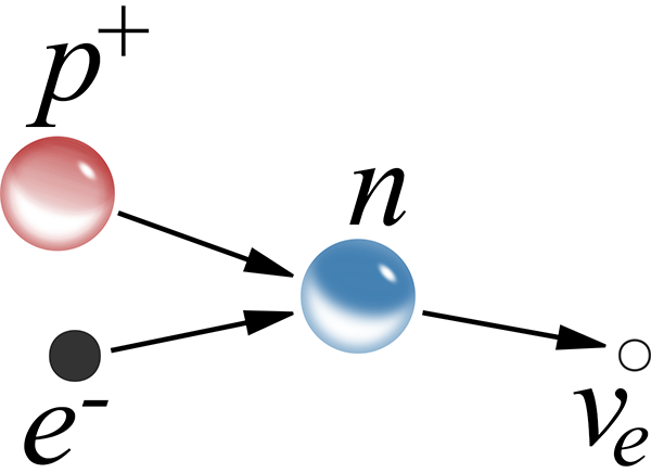
Electron capture. A proton and electron combine to form a neutron. An electron neutrino is emitted in the process.

In most circumstances though, an electron will not approach a proton close enough to combine into a neutron, because there is a quantum mechanical energy barrier between them. The electron is attracted to the proton by electromagnetic force, but if it gets too close then its position becomes increasingly localised and by Heisenberg’s uncertainty principle its energy goes up correspondingly. The minimum energy state is the orbital distance where the electron’s probability distribution is highest. In electron capture, the weak nuclear force overcomes this energy barrier.

Electron capture energy diagram

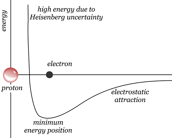
Diagram of electron energy at different distances from a proton. Far away, electrostatic attraction pulls the electron closer, but if it gets too close, Heisenberg uncertainty makes the kinetic energy too large, so the electron settles around the minimum energy distance.

But you can also overcome the energy barrier by providing external energy in the form of pressure. Squeeze the electron and proton enough and you can push through the energy barrier, forcing them to combine into a neutron. In 1934 (less than 2 years after Chadwick discovered the neutron), astronomers Walter Baade and Fritz Zwicky proposed that this could happen naturally, in the cores of large stars following a supernova explosion (previously discussed in the article on supernova 1987A).

During a star’s lifetime, the enormous mass of the star is prevented from collapsing under its own gravity by the energy produced by nuclear fusion in the core. When the star begins to run out of nuclear fuel, that energy is no longer sufficient to prevent further gravitational collapse. Small stars collapse to a state known as a white dwarf, in which the minimal energy configuration has the atoms packed closely together, with electrons filling all available quantum energy states, so it’s not possible to compress the matter further. However, if the star has a mass greater than about 1.4 times the mass of our own sun, then the resulting pressure is so great that it overwhelms the nuclear energy barrier and forces the electrons to combine with protons, forming neutrons. The star collapses even further, until it is essentially a giant ball of neutrons, packed shoulder to shoulder.

These collapses, to a white dwarf or a so-called neutron star, are accompanied by a huge and sudden release of gravitational potential energy, which blows the outer layers of the star off in a tremendously violent explosion, which is what we can observe as a supernova. Baade and Zwicky proposed the existence of neutron stars based on the understanding of physics at the time. However, they could not imagine any method of ever detecting a neutron star. A neutron star would, they imagined, simply be a ball of dead neutrons in space. Calculations showed that a neutron star would have a radius of about 10 kilometres, making them amazingly dense, but correspondingly difficult to detect at interstellar distances. So neutron stars remained nothing but a theoretical possibility for decades.

In July 1967, Ph.D. astronomy student Jocelyn Bell was observing with the Interplanetary Scintillation Array at the Mullard Radio Astronomy Observatory in Cambridge, under the tutelage of her supervisor Antony Hewish. She was looking for quasars – powerful extragalactic radio sources which had recently been discovered using the new observation technique of radio astronomy. As the telescope direction passed through one particular patch of sky in the constellation of Vulpecula, Bell found some strange radio noise. Bell and Hewish had no idea what the signal was. At first they assumed it must be interference from some terrestrial or known spacecraft radio source, but over the next few days Bell noticed the signal appearing 4 minutes earlier each day. It was rising and setting with the stars, not in synch with anything on Earth. The signal was from outside our solar system.

Bell suggested running the radio signal strength plotter at faster speeds to try to catch more details of the signal. It took several months of persistent work, examining kilometres of paper plots. Hewish considered it a waste of time, but Bell persisted, until in November she saw the signal drawn on paper moving extremely rapidly through the plotter. The extraterrestrial radio source was producing extremely regular pulses, about 1 1/3 seconds apart.

PSR B1919+21 trace

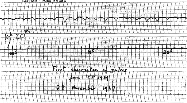
The original chart recorder trace containing the detection signal of radio pulses from the celestial coordinate right ascension 1919. The pulses are the regularly spaced downward deflections in the irregular line near the top. (Reproduced from [1].)

This was exciting! Bell and Hewish thought that it might possibly be a signal produced by alien life, but they wanted to test all possible natural sources before making any sort of announcement. Bell soon found another regularly pulsating radio source in a different part of the sky, which convinced them that it was probably a natural phenomenon.

They published their observations[2], speculating that the pulses might be caused by radial oscillation in either white dwarfs or neutron stars. Fellow astronomers Thomas Gold and Fred Hoyle, however, immediately recognised that the pulses could be produced by the rotation of a neutron star.

Stars spin, relatively leisurely, due to the angular momentum in the original clouds of gas from which they formed. Our own sun rotates approximately once every 24 days. During a supernova explosion, as the core of the star collapses to a white dwarf or neutron star, the moment of inertia reduces in size and the rotation rate must increase correspondingly to conserve angular momentum, in the same way that a spinning ice skater speeds up by pulling their arms inward. Collapsing from stellar size down to 10 kilometres produces an increase in rotation rate from once per several days to the incredible rate of about once per second. At the same time, the star’s magnetic field is pulled inward, greatly strengthening it. Far from being a dead ball of neutrons, a neutron star is rotating rapidly, and has one of the strongest magnetic fields in nature. And when a magnetic field oscillates, it produces electromagnetic radiation, in this case radio waves.

The magnetic poles of a neutron star are unlikely to line up exactly with the rotational axis. Radio waves are generated by the rotation and funnelled out along the magnetic poles, forming beams of radiation. So as the neutron star rotates, these radio beams sweep out in rotating circles, like lighthouse beacons. A detector in the path of a radio beam will see it flash briefly once per rotation, at regular intervals of the order of one second – exactly what Bell observed.

Pulsar diagram

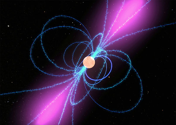
Diagram of a pulsar. The neutron star at centre has a strong magnetic field, represented by field lines in blue. I the star rotates about a vertical axis, the magnetic field generates radio waves beamed in the directions shown by the purple areas, sweeping through space like lighthouse beacons. (Public domain image by NASA, from Wikimedia Commons.)

Radio-detectable neutron stars quickly became known as pulsars, and hundreds more were soon detected. For the discovery of pulsars, Antony Hewish was awarded the Nobel Prize in Physics in 1974, however Jocelyn Bell (now Jocelyn Bell Burnell after marriage) was overlooked, in what has become one of the most notoriously controversial decisions ever made by the Nobel committee.

Jocelyn Bell Building

Image of Jocelyn Bell Burnell on the Jocelyn Bell Building in the Parque Tecnológico de Álava, Araba, Spain. (Public domain image from Wikimedia Commons.)

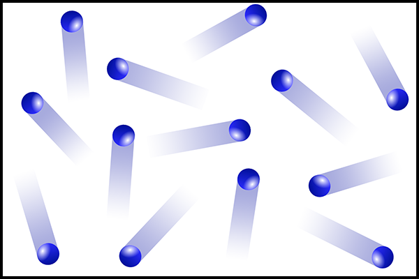
Astronomers found pulsars in the middle of the Crab Nebula supernova remnant (recorded as a supernova by Chinese astronomers in 1054), the Vela supernova remnant, and several others, cementing the relationship between supernova explosions and the formation of neutron stars. Popular culture even got in on the act, with Joy Division’s iconic 1979 debut album cover for Unknown Pleasures featuring pulse traces from pulsar B1919+21, the very pulsar that Bell first detected.

By now, the strongest and most obvious pulsars have been discovered. To discover new pulsars, astronomers engage in pulsar surveys. A radio telescope is pointed at a patch of sky and the strength of radio signals received is recorded over time. The radio trace is noisy and often the pulsar signal is weaker than the noise, so it’s not immediately visible like B1919+21. To detect it, one method is to perform a Fourier transform on the signal, to look for a consistent signal at a specific repetition period. Unfortunately, this only works for relatively strong pulsars, as weak ones are still lost in the noise.

A more sensitive method is called epoch folding, which is performed by cutting the signal trace into pieces of equal time length and summing them all up. The noise, being random, tends to cancel out, but if a periodic signal is present at the same period as the sliced time length then it will stack on top of itself and become more prominent. Of course, if you don’t know the period of a pulsar present in the signal, you need to try doing this for a large range of possible periods, until you find it.

To further increase the sensitivity, you can add in signals recorded at different radio frequencies as well – most radio telescopes can record signals at multiple frequencies at once. A complication is that the thin ionised gas of the interstellar medium slows down the propagation of radio waves slightly, and it slows them down by different amounts depending on the frequency. So as the radio waves propagate through space, the different frequencies slowly drift out of synch with one another, a phenomenon known as dispersion. The total amount of dispersion depends in a known way on the amount of plasma travelled through—known as the dispersion measure—so measuring the dispersion of a pulsar gives you an estimate of how far away it is. The estimate is a bit rough, because the interstellar medium is not uniform – denser regions slow down the waves more and produce greater dispersion.

Pulsar dispersion

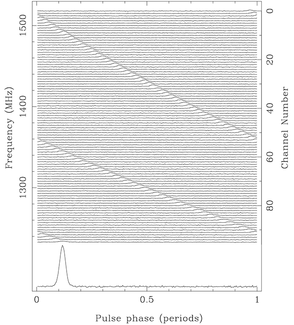
Dispersion of pulsar pulses. Each row is a folded and summed pulse profile over many observation periods, as seen at a different radio frequency. Note how the time position of the pulse drifts as the frequency varies. If you summed these up without correction for this dispersion, the signal would disappear. The bottom trace shows the summed signal after correction for the dispersion by shifting all the pulses to match phase. (Reproduced from [3].)

So to find a weak pulsar of unknown period and dispersion measure, you fold all the signals at some speculative period, then shift the frequencies by a speculative dispersion measure and add them together. Now we have a two-dimensional search space to go through. This approach takes a lot of computer time, trying many different time folding periods and dispersion measures, and has been farmed out as part of distributed “home science” computing projects. The pulsar J2007+2722 was the first pulsar to be discovered by a distributed home computing project[4].

But wait – there’s one more complication. The observed period of a pulsar is equal to the emission period if you observe it from a position in space that is not moving relative to the pulsar. If the observer is moving with respect to the pulsar, then the period experiences a Doppler shift. Imagine you are moving away from a pulsar that is pulsing exactly once per second. A first pulse arrives, but in the second that it takes the next pulse to arrive, you have moved further away, so the radio signal has to travel further, and it arrives a fraction of a second more than one second after the previous pulse. The difference is fairly small, but noticeable if you are moving fast enough.

The Earth moves around the sun at an orbital speed of 29.8 km/s. So if it were moving directly away from a pulsar, dividing this by the speed of light, each successive pulse would arrive 0.1 milliseconds later than if the Earth were stationary. This would actually not be a problem, because instead of folding at a period of 1.0000 seconds, we could detect the pulsar by folding at a period of 1.0001 seconds. But the Earth doesn’t move in a straight line – it orbits the sun in an almost circular ellipse. On one side of the orbit the pulsar period is measured to be 1.0001 s, but six months later it appears to be 0.999 s.

This doesn’t sound like much, but if you observe a pulsar for an hour, that’s 3600 seconds, and the cumulative error becomes 0.36 seconds, which is far more than enough to completely ruin your signal, smearing it out so that it becomes undetectable. Hewish and Bell, in their original pulsar detection paper, used the fact that they observed this timing drift consistent with Earth’s orbital velocity to narrow down the direction that the pulsar must lie in (their telescope received signals from a wide-ish area of sky, making pinpointing the direction difficult).

Timing drift of pulsar B1919+21

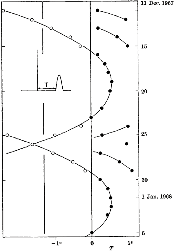
Timing drift of pulsar B1919+21 from Hewish and Bell’s discovery paper. Cumulative period timing difference on the horizontal axis versus date on the vertical axis. If the Earth were not moving through space, all the detection periods for different dates would line up on the 0. With no other data at all, you can use this graph to work out the period of Earth’s orbit. (Figure reproduced from [2].)

What’s more, not just the orbit of the Earth, but also the rotation of the Earth affects the arrival times of pulses. When a pulsar is overhead, it is 6370 km (the radius of the Earth) closer than when it is on the horizon. Light takes over 20 milliseconds to travel that extra distance – a huge amount to consider when folding pulsar data. So if you observe a pulsar over a single six-hour session, the period can drift by more than 0.02 seconds due to the rotation of the Earth.

These timing drifts can be corrected in a straightforward manner, using the astronomical coordinates of the pulsar, the latitude and longitude of the observatory, and a bit of trigonometry. So in practice these are the steps to detect undiscovered pulsars:

  1. Observe a patch of sky at multiple radio frequencies for several hours, or even several days, to collect enough data.
  2. Correct the timing of all the data based on the astronomical coordinates, the latitude and longitude of the observatory, and the rotation and orbit of the Earth. This is a non-linear correction that stretches and compresses different parts of the observation timeline, to make it linear in the pulsar reference frame.
  3. Perform epoch folding with different values of period and dispersion measure, and look for the emergence of a significant signal above the noise.
  4. Confirm the result by observing with another observatory and folding at the same period and dispersion measure.

This method has been wildly successful, and as of September 2019 there are 2796 known pulsars[5].

If step 2 above were omitted, then pulsars would not be detected. The timing drifts caused by the Earth’s orbit and rotation would smear the integrated signal out rather than reinforcing it, resulting in it being undetectable. The latitude and longitude of the observatory are needed to ensure the timing correction calculations are done correctly, depending on where on Earth the observatory is located. It goes almost without saying that the astronomers use a spherical Earth model to get these corrections right. If they used a flat Earth model, the method would not work at all, and we would not have detected nearly as many pulsars as we have.

Addendum: Pulsars are dear to my own heart, because I wrote my physics undergraduate honours degree essay on the topic of pulsars, and I spent a summer break before beginning my Ph.D. doing a student project at the Australia Telescope National Facility, taking part in a pulsar detection survey at the Parkes Observatory Radio Telescope, and writing code to perform epoch folding searches.

Some of the data I worked on included observations of pulsar B0540-69, which was first detected in x-rays by the Einstein Observatory in 1984[6], and then at optical wavelengths in 1985[7], flashing with a period of 0.0505697 seconds. I made observations and performed the data processing that led to the first radio detection of this pulsar[8]. (I’m credited as an author on the paper under my unmarried name.) I can personally guarantee you that I used timing corrections based on a spherical model of the Earth, and if the Earth were flat I would not have this publication to my name.

References:

[1] Lyne, A. G., Smith, F. G. Pulsar Astronomy. Cambridge University Press, Cambridge, 1990.

[2] Hewish, A., Bell, S. J., Pilkington, J. D. H., Scott, P. F., Collins, R. A. “Observation of a Rapidly Pulsating Radio Source”. Nature, 217, p. 709-713, 1968. https://doi.org/10.1038/217709a0

[3] Lorimer, D. R., Kramer, M. Handbook of Pulsar Astronomy. Cambridge University Press, Cambridge, 2012.

[4 Allen, B., Knispel, B., Cordes, J.; et al. “The Einstein@Home Search for Radio Pulsars and PSR J2007+2722 Discovery”. The Astrophysical Journal, 773 (2), p. 91-122, 2013. https://doi.org/10.1088/0004-637X/773/2/91

[5] Hobbs, G., Manchester, R. N., Toomey, L. “ATNF Pulsar Catalogue v1.61”. Australia Telescope National Facility, 2019. https://www.atnf.csiro.au/people/pulsar/psrcat/ (accessed 2019-10-09).

[6] Seward, F. D., Harnden, F. R., Helfand, D. J. “Discovery of a 50 millisecond pulsar in the Large Magellanic Cloud”. The Astrophysical Journal, 287, p. L19-L22, 1984. https://doi.org/10.1086/184388

[7] Middleditch, J., Pennypacker, C. “Optical pulsations in the Large Magellanic Cloud remnant 0540–69.3”. Nature. 313 (6004). p. 659, 1985. https://doi.org/10.1038/313659a0

[8] Manchester, R. N., Mar, D. P., Lyne, A. G., Kaspi, V. M., Johnston, S. “Radio Detection of PSR B0540-69”. The Astrophysical Journal, 403, p. L29-L31, 1993. https://doi.org/10.1086/186714

29. Neutrino beams

We’ve met neutrinos before, when talking about supernova 1987A.

Historically, the early quantum physicist Wolfgang Pauli first proposed the existence of the neutrino in 1930, to explain a problem with then-current understanding of radioactive beta decay. In beta decay, an atomic nucleus emits an electron, which has a negative electric charge, and the resulting nucleus increases in positive charge, transmuting into the element with the next highest atomic number. The law of conservation of energy applied to this nuclear reaction implied that the electron should be emitted from any given isotope with a specific energy, balancing the change in mass as given by Einstein’s famous E = mc2 (energy equals mass times the speed of light squared). Alpha particles emitted during alpha decay, and gamma rays emitted during gamma decay appear at fixed energies.

beta decay, early conception

Illustration of beta decay. The nucleus at left emits an electron. (Public domain image from Wikimedia Commons.)

However, this was not what was observed for beta decay electrons. The ejected electrons had a maximum energy as predicted, but also appeared with a spread of lower energies. Pauli suggested that another particle was involved in the beta decay reaction, which carried off some of the energy. In a three-body reaction, the energy could be split between the electron and the new particle in a continuous fashion, thus explaining the spread of electron energies. Pauli suggested the new particle must be very light, so as to evade detection up to that time. He called it a “neutron”, a neutral particle following the word-ending convention of electron and proton.

However, in the same year German physicists Walther Bothe and Herbert Becker produced some strange radiation by bombarding light elements with alpha particles from radioactive polonium. This radiation had properties unlike other forms known at the time, and several experimenters tried to understand it. In 1932, James Chadwick performed experiments that demonstrated the radiation was made of neutral particles of about the same mass as a proton. The name “neutron” had been floating around nuclear physics for some time (Pauli wasn’t the first to use it; “neutron” appears in the literature as a name for proposed hypothetical neutral particles as early as 1899), but Chadwick was the first experimenter to demonstrate the existence of a neutral particle, so the name got attached to his discovery. Italian physicist Enrico Fermi responded by referring to Pauli’s proposed very light neutral particle as a “neutrino”, or “little neutron” in Italian coinage.

beta decay

Beta decay. A neutron decays to produce a proton, an electron, and an electron anti-neutrino. The neutrino produced has to be an antiparticle to maintain matter/antimatter balance, though it is often referred to simply as a “neutrino” rather than an anti-neutrino. (Public domain image from Wikimedia Commons.)

Detection of the neutrino had to wait until 1956, when a sensitive enough experiment could be performed, by American physicists Clyde Cowan and Frederick Reines, for which Reines received the 1995 Nobel Prize in Physics (Cowan had unfortunately died in 1974). In 1962, Leon Lederman, Melvin Schwartz, and Jack Steinberger of Fermilab discovered that muons—particles similar to electrons but with more mass—had their own associated neutrinos, distinct from electron neutrinos. They received the Nobel Prize for this discovery in 1988 (only a 26 year wait, unlike Reines’ 39 year wait). Finally, Martin Perl discovered a third, even more massive electron-like particle, named the tau lepton, in 1975, for which he shared that 1995 Prize with Reines. The tau lepton, like the electron and muon, has its own distinct associated neutrino.

Meanwhile, other researchers had been building neutrino detectors to observe neutrinos emitted by the sun’s nuclear reactions. Neutrinos interact only extremely weakly with matter, so although approximately 7×10¹⁴ solar neutrinos hit every square metre of Earth every second, almost none of them affect anything, and in fact almost all of them pass straight through the Earth and continue into space without stopping. To detect neutrinos you need a large volume of transparent material; water is usually used. Occasionally one neutrino of the trillions that pass through every second will interact, causing a single-atom nuclear reaction that produces a brief flash of light, which can then be seen by light detectors positioned around the periphery of the transparent material.

Daya Bay neutrino detector

Interior of the Daya Bay Reactor neutrino detector, China. The glassy bubbles house photodetectors to detect the flashes of light produced by neutrino interactions in the liquid filled interior (not filled in this photo). (Public domain image by U.S. Department of Energy, from Wikimedia Commons.)

When various solar neutrino detectors were turned on, there was a problem. They detected only about one third to one half of the number of neutrinos expected from models of how the sun works. The physics was thought to be well understood, so there was great trouble trying to reconcile the observations with theory. One of the least “break everything else we know about nuclear physics” proposals was that perhaps neutrinos could spontaneously and randomly change flavour, converting between electron, muon, and tau neutrinos. The neutrino detectors could only detect electron neutrinos, so if the neutrinos generated by the sun could change flavour (a process known as neutrino oscillation) during the time it took them to arrive at Earth, the result would be a roughly equal mix of the three flavours, so the detectors would only see about a third of them.

Another unanswered question about neutrinos was whether they had mass or not. Neutrinos have only ever been detected travelling at speeds so close to the speed of light that we weren’t sure if they were travelling at the speed of light (in which case they must be massless, like photons) or just a tiny fraction below it (in which case they must have a non-zero mass). Even the neutrinos detected from supernova 1987A, 168,000 light years away, arrived before the initial light pulse from the explosion (because the neutrinos passed immediately out of the star’s core, while the light had to contend with thousands of kilometres of opaque gas before being released), so we weren’t sure if they were travelling at the speed of light or just very close to it. Interestingly, the mass of neutrinos is tied to whether they can change flavour: if neutrinos are massless, then they can’t change flavour, whereas if they have mass, then they must be able to change flavour.

To test these properties, particle physicists began performing experiments to see if neutrinos could change flavour. To do this, you need to produce some neutrinos and then measure them a bit later to see if you can detect any that have changed flavour. But because neutrinos move at very close to the speed of light, you can’t detect them at the same place you create them; you need to have your detector a long way away. Preferably hundreds of kilometres or more.

The first such experiment was the KEK to Kamioka, or K2K experiment, running from 1999-2004. This involved the Japanese KEK laboratory in Tsukuba generating a beam of muon neutrinos and aiming the beam at the Super-Kamiokande neutrino detector at Kamioka, a distance of 250 kilometres away.

K2K map

Map of central Japan, showing the locations of KEK and Super-Kamiokande. (Figure reproduced from [1].)

The map is from the official website of KEK. Notice that Super-Kamiokande is on the other side of a mountain range from KEK. But this doesn’t matter, because neutrinos travel straight through solid matter! Interestingly, here’s another view of the neutrino path from the KEK website:

K2K cross section

Cross sectional view of neutrino beam path from KEK to Super-Kamiokande. (Figure reproduced from [1].)

You can see that the neutrino beam passes underneath the mountains from KEK to the underground location of the Super-Kamiokande detector, in a mine 1000 metres below Mount Ikeno (altitude 1360 m). KEK at Tsukuba is at an altitude of 35 m. Now because of the curvature of the Earth, the neutrino beam passes in a straight line 1000 m below sea level at its middle point. With the radius of the Earth 6367 km, Pythagoras’ theorem tells us that the centre of the beam path is 6365.8 km from the centre of the Earth, so 1200 m below the mean altitude of KEK and Super-Kamiokande – the maths works out. Importantly, the neutrino beam cannot be fired horizontally, it has to be aimed at an angle of about 0.5° into the ground for it to emerge correctly at Super-Kamiokande.

The K2K experiment succeeded in detecting a loss of muon neutrinos, establishing that some of them were oscillating into other neutrino flavours.

A follow up experiment, MINOS, began in 2005, this time using a neutrino beam generated at Fermilab in Illinois, firing at a detector located in the Soudan Mine in Minnesota, some 735 km away.

MINOS map and cross section

Map and sectional view of the MINOS experiment. (Figure reproduced from [2].)

In this case, the straight line neutrino path passes 10 km below the surface of the Earth, requiring the beam to be aimed downwards at an angle of 1.6° in order to successfully reach the detector. Another thing that MINOS did was to measure the time of flight of the neutrino beam between Fermilab and Soudan. When they sent a pulsed beam and measured the time taken for the pulse to arrive at Soudan, then divided it by the distance, they concluded that the speed of the neutrinos was between 0.999976 and 1.000126 times the speed of light, which is consistent with them not violating special relativity by exceeding the speed of light[3].

If you measure the distance from Fermilab to Soudan along the curvature of the Earth, as you would do for normal means of travel (or if the Earth were flat), you get a distance about 410 metres (or 0.06%) longer than the straight line distance through the Earth that the neutrinos took. If the scientists had used that distance, then their neutrino speed measurements would have given values 0.06% higher: 1.00053 to 1.00068 times the speed of light. In other words, to get a result that doesn’t violate known laws of physics, you have to take account of the fact that the Earth is spherical, and not flat.

This result has been reproduced with reduced uncertainty bounds by the CERN Neutrinos to Gran Sasso (CNGS) experiment in Europe, which fires a neutrino beam from CERN in Switzerland to the OPERA detector at the Gran Sasso National Laboratory in Italy.

CNGS cross section

Sectional view of the CNGS experiment neutrino beam path. (Image is Copyright CERN, used under CERN Terms of Use, from [4].)

The difference between the neutrino travel times and the speed of light over the 732 km beam path was measured to be -1.9±3.7 nanoseconds, consistent with zero difference[5]. In this case, if a flat Earth model had been used, the beam path distance would be equal to the surface distance from CERN to Gran Sasso, again about 410 metres longer. This would have given the neutrino travel time difference to be an extra 410/c = 1370 ns, making the neutrinos travel significantly faster than the speed of light.

All of these experiments have shown that neutrino oscillation does occur, which means neutrinos have a non-zero mass. But we still don’t know what that mass is. It must be small enough that for all our existing experiments we can’t detect any any difference between the neutrino speed and the speed of light. More experiments are underway to try and pin down the nature of these elusive particles.

But importantly for our purposes, these neutrino beam experiments make no sense if the Earth is flat, and can only be interpreted correctly because we know the Earth is a globe.

References:

[1] “Long Baseline neutrino oscillation experiment, from KEK to Kamioka (K2K)”. KEK website. http://neutrino.kek.jp/intro/ (accessed 2019-10-01.)

[2] Louis, W. C. “Viewpoint: The antineutrino vanishes differently”. Physics, 4, p. 54, 2011. https://physics.aps.org/articles/v4/54

[3] MINOS collaboration, Adamson, P. et al. “Measurement of neutrino velocity with the MINOS detectors and NuMI neutrino beam”. Physical Review D, 76, p. 072005, 2007. https://doi.org/10.1103/PhysRevD.76.072005

[4] “Old accelerators image gallery”. CERN. https://home.cern/resources/image/accelerators/old-accelerators-images-gallery (accessed 2019-10-01).

[5] The OPERA collaboration, Adam, T., Agafonova, N. et al. “Measurement of the neutrino velocity with the OPERA detector in the CNGS beam”. Journal of High Energy Physics, 2012, p. 93, 2012. https://doi.org/10.1007/JHEP10(2012)093