13. Hydrostatic equilibrium

The theory of gravity is wildly successful in explaining and predicting the behaviours of masses. Isaac Newton’s formulation of gravity (published in his Principia Mathematica in 1686) is a simple formula that works very well for most circumstances of interest to people. When the gravitational potential energy or the velocity of a mass is very large, Albert Einstein’s general relativity (published 1915) is required to correctly determine behaviour. Newton’s gravity is in fact an approximation of general relativity that gives almost exactly the correct answer when the gravitational energy per unit mass is small compared to the speed of light squared, and the velocity is much smaller than the speed of light. For almost all calculation purposes, Newton’s law is sufficiently accurate to be used without worrying about the difference.

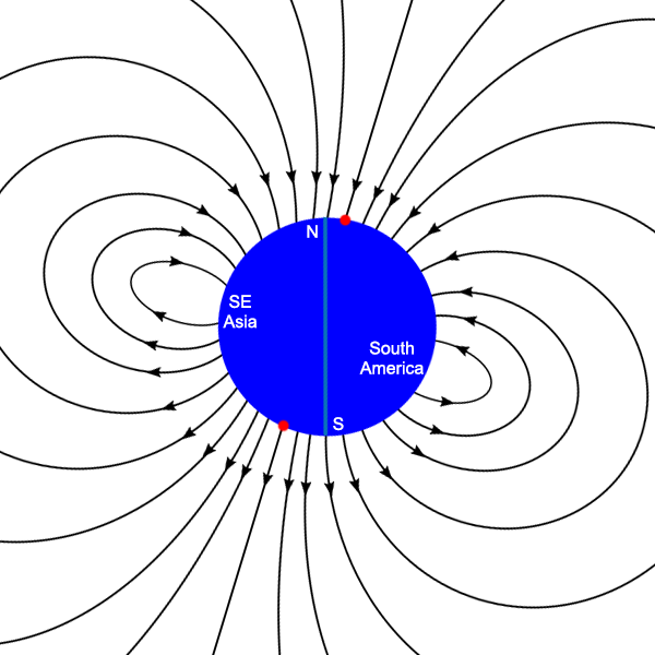
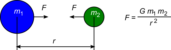
Newton’s law says that the force of gravitational attraction F between two bodies equals the universal gravitational constant G, multiplied by the masses of the two bodies m1 and m2, divided by the square of the distance r between them: F = G m1 m2/(r2).

Newton's law of gravitation

Newton’s law of gravitation describes the force F between two bodies m1 and m2 separated by a distance r between their centres of mass.

Newton himself had no idea why this simple formula worked. Although he showed that it was accurate to the limits of the measurements available to him, he was deeply concerned about its philosophical implications. In particular, he couldn’t imagine how such a force could occur between two bodies separated by any appreciable distance or the vacuum of space. He wrote in a letter to Richard Bentley in 1692:

“That one body may act upon another at a distance through a vacuum without the mediation of anything else, by and through which their action and force may be conveyed from one another, is to me so great an absurdity that, I believe, no man who has in philosophic matters a competent faculty of thinking could ever fall into it.”

Newton was so concerned about this that he added an appendix to the second edition of the Principia – an essay titled the General Scholium. In this he wrote about the distinction between observational, experimental science, and the interpretation of observations (translated from the original Latin):

“I have not as yet been able to discover the reason for these properties of gravity from phenomena, and I do not feign hypotheses. For whatever is not deduced from the phenomena must be called a hypothesis; and hypotheses, whether metaphysical or physical, or based on occult qualities, or mechanical, have no place in experimental philosophy.”

In other words, Newton was being led by his observations to deduce physical laws and how the universe behaves. He refused to countenance speculation unsupported by evidence, and he accepted that the world behaved as observed, even if he didn’t like it. Commenting on Newton’s words in 1840, the philosopher William Whewell wrote:

“What is requisite is, that the hypotheses should be close to the facts, and not connected with them by other arbitrary and untried facts; and that the philosopher should be ready to resign it as soon as the facts refuse to confirm it.”

This affirms the position of a scientist as one who observes nature and tries to describe it as it is. Any hypothesis formed about how things are or why they behave the way they do must conform to all the known facts, and if any future observation contradicts the hypothesis, then the hypothesis must be abandoned (perhaps to be replaced with a different hypothesis). This is the scientific method in a nutshell, and guides our understanding of the shape of the Earth in these pages.

The universal gravitational constant G is a rather small number in familiar units: 6.674×10⁻¹¹ m3 kg−1 s−2. This means that the force of gravity between two everyday objects is so small as to be unnoticeable. For example, even large objects such as two 1-tonne cars a metre apart experience a gravitational force between them of only 6.674×10⁻⁵ newtons – far too small to move the cars against rolling friction, even with the brakes off. Also, the distance between the masses in Newton’s formula is the distance between the centres of mass of the objects, not the closest surfaces. The centres of mass of two cars can’t be brought closer together than about 2 metres in practice, even with the cars touching each other (unless you crush the cars).

Gravity really only starts to significantly affect things when you gather millions of tonnes of mass together. On Earth, the mass of the Earth (5.9722×1024 kilograms) itself dominates our experience with gravity. Removing mass 2 from Newton’s formula, we can calculate the acceleration a towards the centre of mass of the Earth, caused by the Earth’s gravity, as experienced at the surface of the planet (r = 6370 kilometres): a = G m1/(r2) = 6.674×10−11 × 5.9722×1024 / (6370×103)2 = 9.82 m/s2. This number matches experimental observations we can make of the gravity on the surface of the Earth (for example, using a pendulum: see also Airy’s coal pit experiment).

So large object like planets or other astronomical bodies experience a significant gravitational force on parts of themselves. Think about a tall mountain, such as Mount Everest. Let’s estimate the mass of Mount Everest – just roughly will do for our purposes. It is 8848 metres tall, above sea level. Let’s imagine it’s roughly a cone, with sides sloping at 45°. That makes the radius of the base 8848 metres, and its volume is π × 88483 / 3 = 7.25×10¹¹ cubic metres. The density of granite is 2.75 tonnes per cubic metre, so the mass of Mount Everest is roughly 2×10¹⁵ kg. It experiences a gravitational force of approximately 2×10¹⁶ newtons, pulling it down towards the rest of the Earth.

Newton's law of gravitation

Approximating Mount Everest as a cone of rock to calculate the pressure on the base.

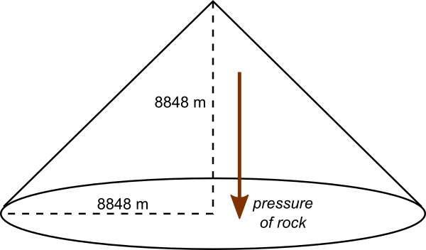
Obviously Mount Everest is strong enough to withstand this enormous force without collapsing. But how much higher could a mountain be without collapsing under its own mass? The taller a mountain gets, the more force pulls it down, but the structural strength of the rock making up the mountain does not increase. At some point there is a limit. Our conical Mount Everest model spreads that mass over an area of π × 88482 square metres. This means the pressure of the rock above on this area is 2×10¹⁶ / (π × 88482) = 8×10⁷ pascals, or 80 megapascals (Mpa). Now, the compressive strength of granite is about 200 MPa. We’re pretty close already! Not to mention that rock can also shear and deform plastically, so we probably don’t even need to get as high as 200 MPa before something bad (or spectacular, depending on your point of view!) happens. A mountain twice as high as Everest would almost certainly be unstable and collapse very quickly.

As mountains get pushed up by tectonic activity, their bases spread out under the pressure of the rock above, so that they can’t exceed the limit of the tallest possible mountain. In practice, it turns out that glaciation also has a significant effect on the maximum height of mountains on Earth, limiting them to something not much higher than Everest [1].

Now, compared to the size of the Earth, even a mountain as tall as Everest is pretty insignificant. It is barely a thousandth of the radius of the planet. It’s often said that if shrunk down to the same size, the Earth would be smoother than a billiard ball. In a sense, this is actually true! Billiard and snooker balls are specified to be 52.5 mm in diameter, with a tolerance of 0.05 mm [2]. That is just under a 500th of the radius, so it would be acceptable to have billiard balls for professional play that are twice as rough as the Earth – although in practice I suspect that billiard balls are manufactured smoother than the quoted tolerance.

So, there is a physical limit to the strength of rock that means that Earth can’t have any protruding lumps of any significant size compared to its radius. Similarly, any deep trenches can’t be too deep either, or else they’ll collapse and fill in due to the gravitational stress on the rock pulling it together. The Earth is spherical in shape (more or less) because of the inevitable interaction of gravity and the structural strength of rock. Any astronomical body above a certain size will also necessarily be close to spherical in shape. The size may vary depending on the materials making up the body: rock is stronger than ice, so icy worlds will necessarily be spherical at smaller sizes than rocky ones.

The phenomenon of large bodies assuming a spherical shape is known as hydrostatic equilibrium, referring to the fact that this is the shape assumed by any body with no resistance to shear forces, in other words fluids. For ice and rock, the resistance to shear force is overcome by gravity for objects of size a few hundred to a thousand or so kilometres in diameter. The asteroid Ceres is a hydrostatic spherical shape, with a diameter of 945 km. On the other hand, Saturn’s moon Iapetus is the largest known object to deviate significantly from hydrostatic equilibrium, with a diameter of 1470 km. Iapetus is almost spherical, but has an unusual ridge of mountains running around its equator, with a height around 20 km – about 1/36 of the moon’s radius.

Iapetus

Iapetus, one of the moons of Saturn, photographed by NASA’s Cassini space probe. (Public domain image by NASA.)

It’s safe to say, however, that any planetary sized object has to be very close to spherical – or spheroidal if rotating rapidly, causing a slight bulge around the equator due to centrifugal force. This is because of Newton’s law of gravity, and the structural strength of rock. Our Earth, naturally, is such a sphere.

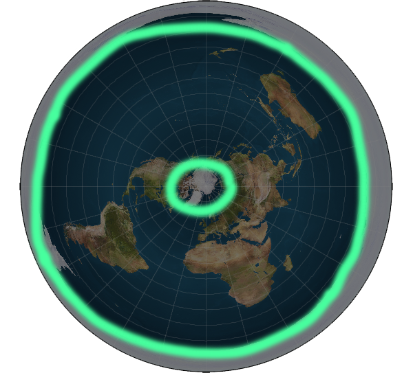
Flat Earth models must either conveniently ignore this conclusion of physics, or posit some otherwise unknown force that maintains the mass of the Earth in a flat, non-spherical shape. By doing so, they violate Newton’s principle that one must be guided by observation, and discard any hypothesis that does not fit the observed facts.

References:

[1] Mitchell, S. G., Humphries, E. E., “Glacial cirques and the relationship between equilibrium line altitudes and mountain range height”. Geology, 43, p. 35-38, 2015. https://doi.org/10.1130/G36180.1

[2] Archived from worldsnooker.com on archive.org: https://web.archive.org/web/20080801105033/http://www.worldsnooker.com/equipment.htm

12. The sun

Possibly the most obvious property of our sun is that it is visible from Earth during daylight hours, but not at night. The visibility of the sun is in fact what defines “day time” and “night time”. At any given time, the half of the Earth facing the sun has daylight, while the other half is in the shadow of the Earth itself, blocking the sun from view. It’s trivial to verify that parts of the Earth are in daylight at the same time as other parts are in night, by communicating with people around the world.

The first physical property of the sun to be measured was how far away it is. In the 3rd century BC, the ancient Greek Aristarchus of Samos (who we met briefly in 2. Eratosthenes’ measurement) developed a method to measure the distance to the sun in terms of the size of the Earth, using the geometry of the relative positions of the sun and moon. Firstly, when the moon appears exactly half-illuminated from a point on Earth, it means that the angle formed by the sun-moon-Earth is 90°. If you observe the angle between the sun and the moon at this time, you can determine the distance to the sun as a multiple of the distance to the moon.

Aristarchus's method 1

Geometry of the sun, moon, and Earth when the moon appears half-illuminated.

In the figure, if you measure the angle θ, then the ratio of the distance to the sun S divided by the distance to the moon M is the reciprocal of the cosine of θ. Aristarchus then used the size of the shadow of Earth on the moon during a lunar eclipse to obtain further equations relating the distances to the sun and moon and the size of the Earth.

Aristarchus's method 2

A medieval copy of Aristarchus’s drawing of the geometry of the sun-Earth-moon system during a lunar eclipse. (Public domain image.)

By combining these results, you can calculate the distances to both the sun and the moon in terms of the radius of the Earth. Aristarchus got the wrong answer, estimating that the sun was only about 19 times further away than the moon, because of the limited precision of his naked eye angle measurements (it’s actually 390 times further away). But Eratosthenes later made more accurate measurements (which were again discussed in Eratosthenes’ measurement), most likely using the same method.

The first rigorous measurement of the absolute distance to the sun was made by Giovanni Cassini in 1672. By this time, observations of all the known celestial bodies in our solar system and some geometry had well and truly established the relative distances of all the orbits. For example, it was known that the orbital radius of Venus was 0.72 times that of Earth, while the orbit of Mars was 1.52 times that of Earth. To measure the absolute distance to the sun, Cassini used a two-step method, the first step of which was measuring the distance to the planet Mars. This is actually a lot easier to do than measuring the distance to the sun, because Mars can be seen at night, against the background of the stars.

Cassini dispatched his colleague Jean Richer to Cayenne in French Guiana, South America, and the two of them arranged to make observations of Mars from there and Paris at the same time. By measuring the angles between Mars and nearby stars, they determined the parallax angle subtended by Mars across the distance between Paris and Cayenne. Simple geometry than gave the distance to Mars in conventional distance units. Then applying this to the relative distances to Mars and the sun gave the absolute distance from the Earth to the sun.

Since 1961, we’ve had a much more direct means of measuring solar system distances. By bouncing radar beams off the moon, Venus, or Mars and measuring the time taken for the signal to return at the speed of light, we can measure the distances to these bodies to high precision (a few hundred metres, although the distances to the planets change rapidly because of orbital motions) [1].

The Earth orbits the sun at a distance of approximately 150 million kilometres. Once we know this, we can work out the size of the sun. The angular size of the sun as seen from Earth can be measured accurately, and is 0.53°. Doing the mathematics, 0.53°×(π/180°)×150 = 1.4, so the sun is about 1.4 million kilometres in diameter, some 109 times the diameter of the Earth. This is the diameter of the visible surface – the sun has a vast “atmosphere” that we cannot see in visible light. Because of its vast distance compared to the size of the Earth, the sun’s angular size does not change appreciably as seen from different parts of the Earth. The difference in angular size between the sun directly overhead and on the horizon (roughly the Earth’s radius, 6370 km, further away) is only about 6370/150000000×(180°/π) = 0.002°.

Our sun is, in fact, a star – a huge sphere composed mostly of hydrogen and helium. It produces energy from mass through well-understood processes of nuclear fusion, and conforms to the observed properties of stars of similar size. The sun appears much larger and brighter than stars, and heats the Earth a lot more than stars, because the other stars are all so much further away.

The Sun

Our sun, observed in the ultraviolet as a false colour image by NASA’s Solar Dynamics Observatory satellite. (Public domain image by NASA.)

Like all normal stars, the sun radiates energy uniformly in all directions. This is expected from the models of its structure, and can be inferred from the uniformity of illumination across its visible disc. The fact that the sun’s polar regions are just as bright as the equatorial edges implies that the radiation we see in the ecliptic plane (the plane of Earth’s orbit) is reproduced in all directions out of the plane as well.

NASA’s Ulysses solar observation spacecraft was launched in 1990 and used a gravity slingshot assist from Jupiter to put it into a solar orbit inclined at about 80° to the ecliptic plane. This allowed it to directly observe the sun’s polar regions.

Ulysses' orbit

Polar orbit of Ulysses around the sun, giving it views of both the sun’s north and south poles. (Public Domain image by NASA.)

Now, I tried to find scientific papers using data from Ulysses to confirm that the sun indeed radiates electromagnetic energy (visible light, ultraviolet, etc.) uniformly in all directions. However, it seems that no researchers were willing to dedicate space in a paper to discussing whether the sun radiates in all directions or not. It’s a bit like looking for a research paper that provides data on whether apples fall to the ground or not. What I did find are papers that use data from Ulyssessolar wind particle flux detectors to measure if the energy emitted by the sun as high energy particles varies with direction.

Solar proton flux versus latitude

Proton flux density observed by Ulysses at various heliographic (sun-centred) latitudes. -90 is directly south of the sun, 0 would be in the ecliptic plane. The track shows Ulysses’ orbit, changing in distance and latitude as it passes under the sun’s south polar regions. Figure reproduced from [2].

Solar wind energy flux versus latitude

Various solar wind plasma component energy fluxes observed by Ulysses at various heliographic latitudes. Figure reproduced from [3].

As these figures show, the energy emitted by the sun as solar wind particles is pretty constant in all directions, from equatorial to polar. Interestingly, there is a variation in the solar wind energy flux with latitude: the solar wind is slower and less energetic close to the plane of the ecliptic than at higher latitudes. The solar wind, unlike the electromagnetic radiation from the sun, is affected by the structure of the interplanetary medium. The denser interplanetary medium in the plane of the ecliptic slows the wind. The amount of slowing provides important constraints on the physics of how the solar wind particles are accelerated in the first place.

Anyway, given there are papers on the variation of solar wind with direction, you can bet your bottom dollar that there would be hundreds of papers about the variation of electromagnetic radiation with direction, if it had been observed, because it goes completely counter to our understanding of how the sun works. The fact that the sun radiates uniformly in all directions is such a straightforward consequence of our knowledge of physics that it’s not even worth writing a paper confirming it.

Now, in our spherical Earth model, all of the above observations are both consistent and easily explicable. In a Flat Earth model, however, these observations are less easily explained.

Why is the sun visible in the sky from part of the Earth (during daylight hours), while in other parts of the Earth at the same time it is not visible (and is night time)?

The most frequently proposed solution for this is that the sun moves in a circular path above the disc of the Flat Earth, shining downwards with a sort of spotlight effect, so that it only illuminates part of the disc. Although there is a straight line view from areas of night towards the position of the sun in the sky, the sun does not shine in that direction.

Given that we know the sun radiates uniformly in all directions, we know this cannot be so. Furthermore, if the sun were a directional spotlight, how would such a thing even come to be? Directional light sources do occur in nature. They are produced by synchrotron radiation from a rapidly rotating object: for example, a pulsar. But pulsars rotate and sweep their directional beams through space on a timescale of approximately one second. If our sun were producing synchrotron radiation, its spotlight beam would be oscillating many times per minute – something which is not observed.

Even furthermore, if the sun is directional and always above the plane of the Flat Earth, it should be visible in the night sky, as an obscuration passing in front of the stars. This prediction of the Flat Earth model is not seen – it is easy to show that no object the size of the sun obscures any stars at night.

And yet furthermore, if the sun is directional, there are substantial difficulties in having it illuminate the moon. Some Flat Earth models acknowledge this and posit that the moon is self-luminous, and changes in phase are caused by the moon itself, not reflection of sunlight. This can easily be observed not to be the case, since (a) there are dark shadows on the moon caused by the light coming from the location of the sun in space, and (b) the moon darkens dramatically during lunar eclipses, when it is not illuminated by the sun.

In addition to the directional spotlight effect, typical Flat Earth models state that the distance to the sun is significantly less than 150 million kilometres. Flat Earth proponent Wilbur Glenn Voliva used geometry to calculate that the sun must be approximately 3000 miles above the surface of the Earth to reproduce the zenith angles of the sun seen in the sky from the equator and latitudes 45° north and south.

Voliva's distance to the sun calculation

Wilbur Glenn Voliva’s calculation that the sun is 3000 miles above the Flat Earth. Reproduced from Modern Mechanics, October 1931, p. 73.

Aside from the fact that Voliva’s distance does not give the correct zenith angles for any other latitudes, it also implies that the sun is only about 32 miles in diameter, given the angular size seen when it is overhead, and that the angular size of the sun should vary significantly, becoming only 0.53°/sqrt(2) = 0.37° when at a zenith angle of 45°. If the sun is this small, there are no known mechanisms than can supply the energy output it produces. And the prediction that the sun would change in angular size is easily disproved by observation.

The simplest and most consistent way of explaining the physical properties of our sun is in a model in which the Earth is a globe.

References:

[1] Muhleman, D. O., Holdridge, D. B., Block, N. “The astronomical unit determined by radar reflections from Venus”. The Astrophysical Journal, 67, p. 191-203, 1962. https://doi.org/10.1086/108693

[2] Barnes, A., Gazis, P. R., Phillips, J. L. “Constraints on solar wind acceleration mechanisms from Ulysses plasma observations: The first polar pass”. Geophysical Research Letters, 22, p. 3309-3311, 1995. https://doi.org/10.1029/95GL03532

[3] Phillips, J. L., Bame, S. J., Barnes, A., Barraclough, B. L., Feldman, W. C., Goldstein, B. E., Gosling, J. T., Hoogeveen, G. W., McComas, D. J., Neugebauer, M., Suess, S. T. “Ulysses solar wind plasma observations from pole to pole”. Geophysical Research Letters, 22, p. 3301-3304, 1995. https://doi.org/10.1029/95GL03094

11. Auroral ovals

Aurorae are visible light phenomena observed in the night sky, mostly at high latitudes corresponding to Arctic and Antarctic regions. An aurora can appear as an indistinct glow from a distance or as distinct shifting curtain-like formations of light, in various colours, when seen from nearby.

An aurora

An aurora, observed near Eielson Air Force Base, near Fairbanks, Alaska. (Public domain image by Senior Airman Joshua Strang, United States Air Force.)

Aurorae are caused by the impact on Earth’s atmosphere of charged particles streaming from the sun, known as the solar wind.

Solar wind and Earth's magnetosphere

Schematic representation of the solar wind streaming from the sun and interacting with the Earth’s magnetic field. The dashed lines indicate paths of solar particles towards Earth. The solid blue lines show Earth’s magnetic field. (Public domain image by NASA.)

The Earth’s magnetic field captures the particles and deflects them (according to the well-known laws of electromagnetism) so that they spiral downwards around magnetic field lines. The result is that the particles hit the atmosphere near the Earth’s magnetic poles.

Solar wind interacting with Earth's magnetosphere

Diagram of the solar wind interacting with Earth’s magnetic field (field lines in red). The magnetic field deflects the incoming particles around the Earth, except for a fraction of the particles that enter the magnetic polar funnels and spiral down towards Earth’s magnetic poles. (Public domain image by NASA. modified.)

The incoming high energy particles ionise nitrogen atoms in the upper atmosphere, as well as exciting oxygen atoms and nitrogen molecules into high energy states. The recombination of nitrogen and the relaxation of the high energy states results in the emission of photons. The light is produced between about 90 km and 150 km above the surface of the Earth, as shown by triangulating the positions of aurorae from multiple observing locations.

Observations of aurorae have established that they occur in nearly-circular elliptical rings of width equivalent to a few degrees of latitude (i.e. a few hundred kilometres), usually between 10° and 20° from the Earth’s magnetic poles. These rings, in the northern and southern hemispheres, are called the auroral ovals.

Northern auroral oval

Northern auroral oval observed on 22 January 2004. Figure reproduced from [1].

The auroral ovals are not precisely centred on the magnetic poles, but rather are pushed a few degrees towards the Earth’s night side. This is caused by the diurnal deflection of the Earth’s magnetic field by pressure from the charged particles of the solar wind.

Northern auroral oval seen by DE-1

Northern auroral oval observed in 1983 by Dynamics Explorer 1 satellite. The large bright patch at left is the daylight side of Earth. (Public domain image by NASA.)

The auroral ovals also expand when solar activity increases, particularly during solar storms, when increased particle emission from the sun and the resulting stronger solar wind compresses the Earth’s magnetic field, forcing field lines to move away from the poles.

But despite these variations, the auroral ovals in the northern and southern hemispheres move and change sizes more or less in unison, and are always of similar size.

Southern auroral oval

Southern auroral oval observed in 2005 by IMAGE satellite, overlaid on a Blue Marble image of Earth. (Public domain image by NASA.)

You can see the current locations and sizes of both the northern and southern auroral ovals as forecast based on the solar wind and interplanetary magnetic field conditions as measured by the Deep Space Climate Observatory satellite at https://www.spaceweatherlive.com/en/auroral-activity/auroral-oval.

Northern and southern auroral ovals

Current northern and southern auroral ovals as forecast by spaceweatherlive.com on 21 April, 2019. The auroral ovals are the same size and shape.

Earth is not the only planet to display aurorae. Jupiter has a strong magnetic field, which acts to funnel the solar wind towards its polar regions in the same way as Earth’s field does on Earth. Jupiter we can establish by simple observation from ground-based telescopes is close to spherical in shape and not a flat disc. Auroral ovals are observed on Jupiter around both the northern and southern magnetic poles, exactly analogously to on Earth: of close to the same size and shape.

Northern auroral ovals on Jupiter

Auroral ovals on Jupiter observed in the northern and southern polar regions by the Hubble Space Telescope, using the Wide Field Planetary Camera (1996) and the Space Telescope Imaging Spectrograph (1997-2001). Figure reproduced from [2].

Similar auroral ovals are also seen on Saturn, in both the northern and southern hemispheres [3][4]. And just for the record, Saturn is also easily shown to be spherical in shape, and not a flat disc.

Now, we have established that auroral ovals appear on three different planets, with the southern and northern ovals of close to the same sizes and shapes on each individual planet. Everything is consistent and readily understandable – as long as you assume that the Earth is spherical like Jupiter and Saturn.

If the Earth is flat, however, then the distributions of aurorae in the north and south map to very different shapes and sizes – with no ready explanation for either the shapes or their differences. In particular, large parts of the southern auroral oval end up being extremely far from the southern magnetic pole, in defiance of the electromagnetic mechanism that causes aurorae in the first place.

Auroral ovals on a flat Earth

Auroral ovals in their observed locations, mapped onto a flat disc Earth. The ovals are vastly different sizes.

So the positions of aurorae on a flat Earth cannot be readily explained by known laws of physics, and they also do not resemble the locations and sizes of auroral ovals as observed on other planets. All of these problems go away and become self-consistent if the Earth is a globe.

References:

[1] Safargaleev, V., Sergienko, T., Nilsson, H., Kozlovsky, A., Massetti, S., Osipenko1, S., Kotikov, A. “Combined optical, EISCAT and magnetic observations of the omega bands/Ps6 pulsations and an auroral torch in the late morning hours: a case study”. Annales Geophysicae, 23, p. 1821-1838, 2005. https://doi.org/10.5194/angeo-23-1821-2005

[2] Grodent, D.,Clarke, J. T., Kim, J., Waite Jr., J. H., Cowley, S. W. H. “Jupiter’s main auroral oval observed with HST‐STIS”. Journal of Geophysical Research, 108, p. 1389-1404, 2003. https://doi.org/10.1029/2003JA009921

[3] Cowley, S. W. H., Bunce, E. J., Prangé, R. “Saturn’s polar ionospheric flows and their relation to the main auroral oval”. Annales Geophysicae, 22, p.1379-1394, 2004. https://doi.org/10.5194/angeo-22-1379-2004

[4] Nichols, J. D., Clarke, J. T., Cowley, S. W. H., Duval, J., Farmer, A. J., Gérard, J.‐C., Grodent, D., Wannawichian, S. “Oscillation of Saturn’s southern auroral oval”. Journal of Geophysical Research, 113, A11205, 2008. https://doi.org/10.1029/2008JA013444

10. The Sagnac effect

Imagine beams of light coming from an emitter and travelling around a circular path in both directions, until they arrive back at the source. Such an arrangement can be constructed by using an optic fibre in a circular loop, injecting light at both ends. The distance travelled by the clockwise beam is the same as the distance travelled by the anticlockwise beam, and the speed of light in both directions is the same, so the time taken for each beam to travel from the source back to the origin is the same. So far, so good.

A light loop

A loop with light travelling in both directions.

Now imagine the whole thing is rotating – let’s say clockwise. For reference we’ll use the numbers on a clock face and the finer divisions into 60 minutes. The optic fibre ring runs around the edge of the clock, with the light source and a detector at 12. Now imagine that the clock rotates fast enough that by the time the clockwise-going light reaches the original 12 position, the clock has rotated so that 12 is now located at the original 1 minute past 12 position. The light has to travel an extra 60th of the circle to reach its starting position (actually a tiny bit more than that because the clock is still rotating and will have gone a tiny bit further by the time the light beam catches up). But the light going anticlockwise reaches the source early, only needing to travel a tiny bit more than 59/60 of the circle. The travel times of the two beams of light around the circle are different.

A rotating light loop

Now the loop is rotating. By the time the light has travelled around the loop, the exit from the loop has moved a little bit clockwise. So the light travelling clockwise has to travel further to reach the exit, while the light travelling anticlockwise reaches the exit sooner.

This is a very simplified explanation, and figuring out the mathematics of exactly what happens involves using special relativity, since the speed of light is involved, but it can be shown that there is indeed a time difference between the travel times of beams of light heading in opposite directions around a rotating loop. The time difference is proportional to the speed of rotation and to the area of the loop (and to the cosine of the angle between the rotation axis and the perpendicular to the loop, for those who enjoy vector mathematics). This effect is known as the Sagnac effect, named after French physicist Georges Sagnac, who first demonstrated it in 1913.

Measuring the minuscule time difference between the propagation of the light beams is not difficult, due to the wave nature of light itself. The wavelength of visible light is just a few hundred nanometres, so even a time difference of the order of 10-16 seconds can be observed because it moves the wave crests and troughs of the two beams relative to one another, causing visible interference patterns as they shift out of synchronisation. This makes the device an interferometer that is very sensitive to rotational speed.

The Sagnac effect can be seen not only in a circular loop of optic fibre, but also with any closed loop of light beams of any shape, such as can be constructed with a set of mirrors. This was how experimenters demonstrated the effect before the invention of optic fibres. Because the paths of the two beams of light are the same, just reversed, a Sagnac interferometer is completely insensitive to mechanical construction tolerances, and only sensitive to the physical rotation of the device.

Sagnac actually performed the experiment in an attempt to prove the existence of the luminiferous aether, a hypothetical medium permeating all space through which light waves propagate. He believed his results showed that such an aether existed, but Max von Laue and Albert Einstein showed that Sagnac’s effect could be explained by special relativity, without requiring any aether medium for light propagation.

The interesting thing about the Sagnac effect is that it measures absolute rotational speed, that is: rotation relative to an inertial reference frame, in the language of special relativity. In practice, this means rotation relative to the “fixed” position of distant stars. This is useful for inertial guidance systems, such as those found on satellites, modern airliners and military planes, and missiles. The Sagnac effect is used in ring laser gyroscopes and fibre optic gyroscopes to provide an accurate measure of rotational speed in these guidance systems. GPS satellites use these devices to ensure their signals are correctly calibrated for rotation – without them GPS would be less accurate.

Because the magnitude of the Sagnac effect depends on both the rotational speed and the area of the light loop, by making the area large you can make the interferometer incredibly sensitive to even very slow rotation. Rotations as slow as once per 24 hours. You can use these devices to measure the rotation of the Earth.

This was first done in 1925. Albert A. Michelson (of the famous Michelson-Morley experiment that disproved the existence of the luminiferous aether), Henry G. Gale, and Fred Pearson acquired the use of a tract of land in Clearing, Illinois (near Chicago’s Midway Airport), and built a huge Sagnac interferometer, a rectangle 610×340 metres in size [1][2].

Michelson’s Sagnac interferometer

Diagram of Michelson’s Sagnac interferometer in Clearing, Illinois. The Sagnac loop is defined by the mirrors ADEF. The smaller rectangle ABCD was used for calibration measurements. Light enters from the bottom towards the mirror A, which is half-silvered, allowing half the light through to D, and reflecting half in the other direction towards F. The beams complete circuits ADEF and AFED, returning to A, where the half-silvering reflects the beam from D and lets through the beam from F towards the detector situated outside the loop at the left. The light paths are inside a pipe system, which is evacuated using a pump to remove most of the air. (Figure reproduced from [2].)

With this enormous area, the shift in the light beams caused by the rotation speed of the Earth at the latitude of Chicago was around one fifth of a wavelength of the light used – easily observable. The Michelson-Gale-Pearson experiment’s measurements and calculations showed that the rotation speed they measured was consistent with the rotation of the Earth once every 23 hours and 56 minutes – a sidereal day (i.e. Earth’s rotation period relative to the stars; this is shorter than the average of 24 hours rotation relative to the sun, because the Earth also moves around the sun).

Now the interesting thing is that the Sagnac effect measures the linear rotation speed, not the angular rotation rate. The Earth rotates once per day – that angular rotation rate is constant for the entire planet, and can be modelled in a flat Earth model simply by assuming the Earth is a spinning disc, like a vinyl record or Blu-ray disc. But the linear rotation speed of points on the surface of the Earth varies.

In the typical flat Earth model with the North Pole at the centre of the disc, the rotation speed is zero at the North Pole, and increases linearly with distance from the Pole. As you cross the equatorial regions, the rotational speed just keeps increasing linearly, until it is maximal in regions near the “South Pole” (wherever that may be).

Rotation speed on a flat disc Earth

Rotation speeds at different places on a flat rotating disc Earth (top view of the disc).

On a spherical Earth, in contrast, the rotation speed is zero at the North Pole, and varies as the cosine of the latitude as you travel south, until it is a maximum at the equator, then drops again to zero at the South Pole.

Rotation speed on a flat disc Earth

Rotation speeds at different places on a spherical Earth.

Here is a table of rotation speeds for the two models:

Latitude Speed (km/h)
Flat model
Speed (km/h)
Spherical model
90°N (North Pole) 0.0 0.0
60°N 875.3 837.2
41.77°N (Clearing, IL) 1407.2 1248.9
30°N 1750.5 1450.1
0° (Equator) 2625.8 1674.4
30°S 3501.1 1450.1
45.57°S (Christchurch) 3896.6 1213.3
60°S 4376.4 837.2
90°S (South Pole) 5251.6 0.0

In the Michelson-Gale-Pearson experiment, the calculated expected interferometer shift was 0.236±0.002 of a fringe (essentially a wavelength of the light used), and the observed shift was 0.230±0.005 of a fringe. The uncertainty ranges overlap, so the measurement is consistent with the spherical Earth model that they used to calculate the expected result.

If they had used the North-Pole-centred flat Earth model, then the expected shift would have been 1407.2/1248.9 larger, or 0.266±0.002 of a fringe. This is well outside the observed measurement uncertainty range. So we can conclude that Michelson’s original 1925 experiment showed that the rotation of the Earth is inconsistent with the flat Earth model.

Nowadays we have much more than that single data point. Sagnac interferometers are routinely used to measure the rotation speed of the Earth at various geographical locations. In just one published example, a device in Christchurch, New Zealand, at a latitude of 43°34′S, measured the rotation of the Earth equal to the expected value (for a spherical Earth) to within one part in a million [3]. Given that the expected flat Earth model speed is more than 3 times the spherical Earth speed at this latitude—and all of the other rotation speed measurements made all over the Earth consistent with a spherical Earth—we can well and truly say that any rotating disc flat Earth model is ruled out by the Sagnac effect.

References:
[1] Michelson, A. A. “The Effect of the Earth’s Rotation on the Velocity of Light, I.” The Astrophysical Journal, 61, 137-139, 1925. https://doi.org/10.1086%2F142878
[2] Michelson, A. A.; Gale, Henry G. “The Effect of the Earth’s Rotation on the Velocity of Light, II.” The Astrophysical Journal, 61, p. 140-145, 1925. https://doi.org/10.1086%2F142879
[3] Anderson, R.; Bilger, H. R.; Stedman, G. E. “ “Sagnac” effect: A century of Earth‐rotated interferometers”. American Journal of Physics, 62, p. 975-985, 1994. https://doi.org/10.1119/1.17656

9. The South Pole

One of the most popular models for a flat Earth presumes the Earth to be a circular disc centred at the North Pole, and with Antarctica spanning the rim and providing some form of impassable barrier to simply travelling off the disc.

Disc shaped flat Earth

A common Flat Earth model: a flat circular disc centred at the North Pole. (Public domain image from Wikimedia Commons.)

This raises the question of where the South Pole is. In such a disc model, there is no single South Pole – all points on the rim of the disc are equally far south. Yet people have travelled to a single geographic place that matches all of the physical requirements of being the South Pole of a spherical Earth:

1. People heading south always end up at this same spot, no matter which line of longitude they head south along.

2. At this place, the sun circles the horizon once per 24 hour period during the southern hemisphere summer, not setting until the autumn equinox, after which it circles below the horizon throughout the southern winter, only rising again at the spring equinox. This is exactly as expected for a physical South Pole on a spherical planet.

3. The place is directly underneath the point in the sky around which the southern stars appear to revolve, in a manner exactly analogous to the movement of the stars at the North Pole, but in the opposite rotational direction. The stars at the North Pole appear to rotate anticlockwise in the sky, while at the South Pole they rotate clockwise in the sky.

Star trails in the southern hemisphere

Star trails in the southern hemisphere, photographed in the Atacama Desert in Chile. (Creative Commons Attribution 4.0 International image by the European Southern Observatory.) This photo shows the motion of the southern hemisphere stars through several hours of a night, moving in apparent circles around the South Celestial Pole (the point directly above the Earth’s South Pole). I tried to find a copyright or royalty-free photo of star trails photographed from the South Pole itself, but could not find any, however Astronomy Picture of the Day has such a photo taken at the South Pole, showing complete circles over a 24-hour period of darkness.

Furthermore, from this place, or areas around it, there are no directions in which one cannot travel. There is no visible edge of the disc, nor any impassable barrier to travel.

The same argument applies to the North Pole if the flat Earth is supposed to be a disc with the South Pole at its centre. And if the disc is some other configuration, then there will always be some point on the spherical Earth that ends up corresponding to all the points around the rim of the flat disc Earth – where it is straightforward to travel to that point on the spherical Earth but which is unreachable or should display bizarre properties (such as a rim or impassable barrier) on the flat Earth.

All of this is difficult to explain in a flat Earth model, but is a natural consequence of a spherical Earth.

2.c Eratosthenes and the Flat Earth model

A reader has pointed out that we can also use the data collected in our Eratosthenes experiment to test the hypothesis that the Earth is flat and that the difference in shadows is caused by the sun being a relatively small distance from the flat Earth. And we can compare this test to a test of our round Earth hypothesis.

If the Earth is flat, and we make an observation like Eratosthenes, that a vertical stick in one location casts no shadow, while a vertical stick some distance north (or south) does cast a shadow, then we can use geometry to figure out how far away the sun must be.

Distance to the sun in a flat Earth model

Using similar triangles to determine the distance from a flat Earth to the sun, given an observation of the shadow of a vertical stick, and knowing the distance from a point where the sun is overhead.

If the Earth is indeed flat then when we do this calculation for each of our 19 observations we should get the same answer, to within any experimental error. In particular, there should be no systematic difference in our answers that depends on the distance from the equator. Analogously, in our round Earth model, the circumference we have calculated for the Earth from each of our observations should also be the same to within experimental errors, and show no systematic difference depending on distance from the equator.

So let’s test those things! Here are graphs of the results, on which I’ve included a linear least squares best fit line, showing the line’s equation and statistical R2 score. The R2 value, or coefficient of determination, is a measure of how likely the data values (the circumference of the Earth in the round Earth hypothesis, or the distance to the sun in the flat Earth hypothesis) are to be correlated with the fixed values (the distance from the equator in both cases). We’ll discuss that after we see the data.

Earth's circumference versus distance from equator

Plot of 19 measurements of the Earth’s circumference, assuming the round Earth model, versus distance from the equator.

Distance to sun versus distance from equator

Plot of 19 measurements of the distance of the sun from Earth, assuming the flat Earth model, versus distance from the equator.

The first thing to notice is that in the top plot, the circumference of the Earth values look fairly evenly scattered around the true value. In the bottom plot, the calculated values for the distance of the sun from Earth are not evenly scattered; they show a pretty clear trend of giving larger distances for the data points closer to the equator and smaller distances for data points further from the equator. We can quantify this by looking at the straight line fits to the data and in particular the R2 value.

To do a rigorous statistical test, we need to set up our two possible null hypotheses. These are statements that for the purpose of our statistical test we assume are true, and then we calculate the probability that what we observe could happen by random chance. Our two null hypotheses are:

1. For the spherical Earth model, the calculated circumference of Earth is independent of the distance from the equator of our data points.

2. For the flat Earth model, the calculated distance of the sun from Earth is independent of the distance from the equator of our data points.

To test these, we use a probability distribution that tells us how likely our observed R2 scores are. An appropriate one to use is Student’s t-distribution. We calculate Student’s t-distribution function for 19 data points and 2 degrees of freedom (the y-intercept and the slope of our fitted line), determine a value for the function below which 95% of the probability distribution lies, and convert this to an R2 value using the known transformation. In simpler terms (TL;DR), we’re working out a number R2(P<0.05) which, if our calculated values are independent of distance from the equator, then we would expect 95% of experiments to give an R2 value less than the number R2(P<0.05).

Doing the maths, our value for R2(P<0.05) is 0.334. What this means is that if our R2 value is greater than 0.334, then we should reject our null hypothesis – the data are statistically inconsistent with the hypothesis (at the 95% confidence level, for those who like statistical rigour*). On the other hand, if our R2 value is less than 0.334, we cannot reject our null hypothesis – we haven’t proven it to be true, we have just shown that our data are consistent with it.

Now let’s look at our calculated R2 values. For the spherical Earth hypothesis, R2 = 0.1358. This is less than the critical value, so our data are consistent with our hypothesis. In contrast, for the flat Earth model, R2 = 0.9162. This is greater than the critical value, so we can confidently reject the flat Earth hypothesis as inconsistent with our experiment!

So there you have it. Not only did we successfully measure the circumference of the Earth to within our experimental errors, we have now also shown that our experimental results are consistent with a spherical Earth model, and inconsistent with a flat Earth model.

* Note: Choosing the 95% confidence level is typical for statistical hypothesis testing. You should always choose your confidence level before performing the calculations, to avoid any bias in your reporting. You can choose other levels, such as 99%. If I’d done that, we would have found that our data are also inconsistent with the flat Earth model at the more stringent 99% confidence level. In fact, calculating backwards, the confidence level of our rejection is a bit above 99.7%.

8. Earth’s magnetic field

Magnetic fields have both a strength and a direction at each point in space. The strength is a measure of how strong a force a magnet feels when in the field, and the direction is the direction of the force on a magnetic north pole. North poles of magnets on Earth tend to be pulled towards the Earth’s North Magnetic Pole (which is in fact a magnetic south pole, but called “the North Magnetic Pole” because it is in the northern hemisphere), while south poles are pulled towards the South Magnetic Pole (similarly, actually a magnetic north pole, called “the South Magnetic Pole” because it’s in the south). Humans have used this property of magnets for thousands of years to navigate, with magnetic compasses.

The simplest magnetic field is what’s known as a dipole, because it has two poles: a north pole and a south pole. You can think of this as the magnetic field of a simple bar magnet. The magnetic field lines are loops, with the field direction pointing out of the north pole and into the south pole, and the loops closing inside of the magnet.

A magnetic dipole

Illustration of magnetic field lines around a magnetic dipole. The north and south poles of the magnet are marked.

It’s straightforward to measure both the strength and the direction of the Earth’s magnetic field at any point on the surface, using a device known as a magnetometer. So what does it look like? Here are some contour maps showing the Earth’s magnetic field strength and the inclination – the angle the field lines make to the ground.

Earth's magnetic field intensity

Earth’s magnetic field strength. The minimum field strength occurs over South America; the maximum field strengths occur just off Antarctica, south of Australia, and in the broad patch covering both central Russia and northern Canada. (Public domain image by the US National Ocean and Atmospheric Administration.)

Earth's magnetic field inclination

Earth’s magnetic field inclination. The field direction is parallel to the ground at points along the green line, points into the ground in the red region, and points out of the ground in the blue region. The field emerges vertically at the white mark off the coast of Antarctica, south of Australia – this is the Earth’s South Magnetic Pole. The field points straight down at the North Magnetic Pole, north of Canada – not shown in this Mercator projection map, which omits areas with latitude greater than 70° north or south. (Public domain image by the US National Ocean and Atmospheric Administration.)

Now, how can we explain these observations with either a spherical Earth or flat Earth model? Let’s start with the spherical model.

You may notice a few things about the maps above. The Earth’s magnetic field is not symmetrical at the surface. The lowest intensity point over South America is not mirrored anywhere in the northern hemisphere. And the South Magnetic Pole is at a latitude about 64°S, while the North Magnetic Pole is at latitude 82°N. As it happens, this observed magnetic field is to a first approximation the field of a magnetic dipole – just not a dipole that is centred at the centre of the Earth. The dipole is tilted with respect to Earth’s rotation, and is offset a bit to one side – towards south-east Asia and away from South America. This explains the minimum intensity in South America, and the asymmetry of the magnetic poles.

A magnetic dipole

The Earth’s magnetic field is approximated by a dipole, offset from the centre of the Earth. The rotational axis is the light blue line, with geographic north and south poles marked. The red dots are the equivalent magnetic poles. The North Magnetic Pole is much closer to the geographic north pole than the South Magnetic Pole is to the geographic south pole. (As stated in the text, the “North Magnetic Pole” of the Earth is actually a magnetic south pole, and vice versa.)

Models of the interior of the Earth suggest that there are circulating electrical currents in the molten core, which is composed mostly of iron. These currents are caused by thermal convection, and twisted into helices by the Coriolis force produced by the Earth’s rotation, both well understood physical processes. Circulating electrical currents are exactly what causes magnetic fields. The simplest version of this so-called dynamo theory model is one in which there is a single giant loop of current, generating a simple magnetic dipole. And in fact this dipole fits the Earth’s magnetic field to an average deviation of 16% [1].

This is not a perfect fit, but it’s not too bad. The adjustments needed to better fit Earth’s measured field are relatively small, and can also be understood as the effects of circulating currents in the Earth’s core, causing additional components of the field with smaller magnitudes. (The Earth’s magnetic field also changes over time, but we’ll discuss that another day: Now available in Proof 44. Magnetic striping.)

If the Earth is flat, however, there is no such relatively simple way to understand the strength and direction of Earth’s magnetic field using standard electromagnetic theory. Even the gross overall structure—which is readily explained by a magnetic dipole for the spherical Earth—has no such simple explanation. The shape of the field on a flat Earth would require either multiple electrical dynamos or large deposits of magnetic materials under the Earth’s crust, and they would have to be fortuitously arranged in such a way that they closely mimic a dipole if we assumed the Earth to be a sphere. For any random arrangement of magnetic field-inducing structures on a flat Earth to happen to mimic the field of a spherical planet so closely is highly unlikely. Potentially it could happen, but the Earth actually being a sphere is a much more likely explanation.

That the simpler model is more likely to be true than the one requiring many ad-hoc assumptions is a case of Occam’s razor. In science, particularly, a simpler theory is more easily testable than one with a large number of ad-hoc assumptions. Occam’s razor will come up a lot, and I should probably write a sidebar article about it.

References:

[1] Nevalainen, J.; Usoskin, I.G.; Mishev, A. “Eccentric dipole approximation of the geomagnetic field: Application to cosmic ray computations”. Advances in Space Research, 52, p. 22-29, 2013. https://doi.org/10.1016/j.asr.2013.02.020

2.b Eratosthenes’ measurement results

Thank you to everyone who participated in our measurement of the Earth using Eratosthenes’ method! And thank you to those who tried but were frustrated by the weather – I received several reports of bad weather from the UK, France, and parts of the USA. But we have collected 19 successful observations, from 7 countries: New Zealand, Australia, Israel, Germany, Norway, USA, and Canada. I’ve plotted the locations of the observations on the following map.

Map of measurement locations

Map of observation locations. 16 locations are plotted; 3 of the 19 measurements were taken in the same city as another measurement.

The reason we did this experiment on the date of the equinox (20/21 March) is because that is when the sun is directly over the equator. Rather than use ancient Syene in Egypt as our reference point, where the sun is directly overhead on the summer solstice, we’re doing our calculations based on distance from the equator.

Ideally, I’d have asked all of you to measure the length of your vertical stick, the length of its shadow, and the distance you are away from the nearest point where your stick cast no shadow (which would be on the equator either due south or north of your location). Although in principle you can measure your distance from this point by travelling due south or north to the equator and keeping an accurate log of distance travelled, this would almost certainly have lowered the participation numbers! So as a proxy, I asked for your locations – either the city, or an accurate reading of your latitude from a GPS unit or Google Maps or something similar. This is really just a shortcut so that I can calculate your distance from the equator. And yes, although the existence of “degrees of latitude” is based on the premise that the Earth is spherical, the simple multiplicative relationship between distance and the numbers we call “latitude” still holds in the real world (even if the Earth is flat).

Some summary statistics:

  • Number of data points: 19
  • Shortest distance from equator: 3196 km (Geraldton, Australia)
  • Longest distance from equator: 6662 km (Oslo, Norway)
  • Shortest stick used: 31.5 cm
  • Longest stick used: 250.2 cm

The calculations proceeded as follows:

1. For each location, I calculated the distance from the equator, using the provided latitude.

2. I calculated the angle of the stick’s shadow from the vertical: shadow angle = arctangent(shadow length / stick length).

3. I calculated the circumference of the Earth for each measurement: circumference = 4 × distance from equator × 90°/(shadow angle). Here is a graph of the resulting 19 measurements of the Earth’s circumference, plotted against the length of the stick used in each case.

Map of measurement locations

Plot of 19 measurements of the Earth’s circumference, versus shadow stick length. As the sticks get longer, the results tend to get more accurate, because it is easier to measure the length of the shadow to a smaller percentage error.

4. I calculated the average of the 19 different measurements of circumference, as well as the standard error of the mean, a statistical measure of the expected uncertainty in the average value. (In experiments like this, where we take multiple independent measurements of the same value, we expect there to be some random errors in each result, caused by slight inaccuracies in measuring the lengths of the sticks and shadows. Our best overall estimate is the average of the results, and the amount of scatter in the results can be used to estimate the likely size of any error in the average.)

The result we achieved is that we measured the circumference of the Earth to be 39926 km, with a standard error of 163 km, or (39926 ± 163) km. What this means is that statistically we expect the true value to lie somewhere between 39763 km and 40089 km.

The polar circumference of the Earth is in fact 40008 km, which lies neatly within this range. So we did it! We measured the circumference of the Earth, and we got the right answer to within the statistical uncertainty of our method!

In one small wrinkle, when everyone was reporting their measurements to me, one person reported that his measurement might be a little bit wrong, because he didn’t have access to a level or any other means of ensuring that his stick was exactly vertical when he took the measurement. So he was unsure whether his data should really be included or not. As it turns out, his data produced the measurement with the largest error, the lowest data point on the graph. If we remove his measurement, our average and standard error become: (40012 ± 147) km. Our average is now even closer to the correct answer, a mere 4 km different. If we made many more measurements, being careful to minimise our random errors, we could expect our result to be even better.

So thank you again to all who participated. Now you can honestly brag that you have measured the size of the Earth!