16. Lunar eclipses

Lunar eclipses occur when the Earth is positioned between the sun and the moon, so that the Earth blocks some or all of the sunlight from directly reaching the moon. Because of the relative sizes of the sun, Earth, and moon, and their distances from one another, the Earth’s shadow is large enough to completely cover the moon.

To talk about eclipses, we need to define some terms. The sun is a large, extended source of light, not a point source, so the shadows that objects cast in sunlight have two components: the umbra, where light from the sun is totally blocked, and the penumbra, where light from the sun is partially blocked.

Umbra and penumbra

Diagram showing the umbra and penumbra cast by the Earth. Not to scale. Public domain image from Wikimedia Commons.

When the moon passes entirely inside the Earth’s umbra, that is a total lunar eclipse. Although no sunlight reaches the moon directly, the moon is not completely dark, because some sunlight refracts (bends) through the Earth’s atmosphere and reaches the moon. This light is red for the same reason that sunsets on Earth tend to be red: the atmosphere scatters blue light more easily than red, so red light penetrates large distances of air more easily. This is why during a total lunar eclipse the moon is a reddish colour. Although a totally eclipsed moon looks bright enough to our eyes, it’s actually very dark compared to a normal full moon. Our eyes are very good at compensating for the different light levels without us being aware of it.

Total lunar eclipse

Total lunar eclipse of 28 August 2007 (photographed by me). 1 second exposure at ISO 800 and aperture f/2.8.

The amount of refracted light reaching the moon depends on the cleanliness of the Earth’s atmosphere. If there have been recent major volcanic eruptions, then significantly less light passes through to reach the moon. The brightness of the moon during a total lunar eclipse can be measured using the Danjon scale, ranging from 0 for very dark eclipses, to 4 for the brightest ones. After the eruption of Mount Pinatubo in the Philippines in 1991, the next few lunar eclipses were extremely dark, with the eclipse of December 1992 rating a 0 on the Danjon scale.

When the moon is only partly inside the Earth’s umbra, that is a partial lunar eclipse. A partial phase occurs on either side of a total lunar eclipse, as the moon passes through the Earth’s shadow, and it can also occur as the maximal phase of an eclipse if the moon’s orbit isn’t aligned to carry it fully within the umbra. During a partial eclipse phase, you can see the edge of the Earth’s umbral shadow on the moon.

Partial lunar eclipse phase

Partial phase of the same lunar eclipse of 28 August 2007. 1/60 second exposure at ISO 100 and f/8, which is 1/3840 the exposure of the totality photo above. If this photo was 3840 times as bright, the dark part at the bottom would look as bright as the totality photo (and the bright part would be completely washed out).

Lunar eclipses can only occur at the full moon – those times when the sun and moon are on opposite sides of the Earth. The moon orbits the Earth roughly once every 29.5 days and so full moons occur every 29.5 days. However, lunar eclipses occur only two to five times per year, because the moon’s orbit is tilted by 5.1° relative to the plane of the Earth’s orbit around the sun. This means that sometimes when the moon is full it is above or below the Earth’s shadow, rather than inside it.

Okay, so what can lunar eclipses tell us about the shape of the Earth? A lunar eclipse is a unique opportunity to see the shape of the Earth via its shadow. A shadow is the same shape as a cross-section of the object casting the shadow. Let’s have another look at the shape of Earth’s shadow on the moon, in a series of photos taken during a lunar eclipse:

Lunar eclipse montage

Montage of photos taken over 83 minutes during the lunar eclipse of 28 August 2007. Again, the bottom row of photos have 3840 times the exposure of the top row, so the eclipsed moon is nearly 4000 times dimmer than the full moon.

As you can see, the edge of the Earth’s shadow is curved. The fact that the moon’s surface is curved doesn’t affect this, because we are looking from the same direction as the Earth, so we see the same cross-section of the moon. (Your own shadow looks the shape of a person to you, even if it falls on an irregular surface where it looks distorted to someone else.) So from this observation we can conclude that the edge of the Earth is rounded.

Many shapes can cause a rounded shadow. However, if you observe multiple lunar eclipses, you will see that the Earth’s shadow is always round, and what’s more, it always has the same radius of curvature. And different lunar eclipses occur at any given location on Earth with the moon at different points in the sky, including sometimes when the moon is not in the sky (because the location is facing away from the moon). This means that different lunar eclipses occur when different parts of the Earth are facing the moon, which means that different parts of the Earth’s edge are casting the shadow edge on the moon. So from these observation, we can see that the shape of the shadow does not depend on the orientation of the Earth to the moon.

There is only one solid shape for which the shape of its shadow doesn’t depend on the object’s orientation. A sphere. So observations of lunar eclipses show that the Earth is a globe.

Addendum: A common rebuttal by Flat Earthers is that lunar eclipses are not caused by the Earth’s shadow, but by some other mechanism entirely – usually another celestial object getting between the sun and moon and blocking the light. But any such object is apparently the same colour as the sky, making it mysteriously otherwise completely undetectable, and does not have the simple elegance of explanation (and the supporting evidence from numerous other observations) of the moon moving around the Earth and entering its shadow.

15. Trilateration

Trilateration is the method of locating points in space based on measuring the distances from known reference locations. It is used in surveying and navigation, similarly to the related method of triangulation, which technically uses the measurement of angles, not distances. For this entry we’re going to get practical and attempt to do some trilateration, using distances between some major cities in the world. To do this, I’ll need some equipment:

Equipment used

I acquired graph paper, a ruler, a tape measure, a pen, a pair of compasses, and a couple of large polystyrene balls.

I began my first scale drawing on a piece of graph paper. I’ve picked Auckland, New Zealand, as one of my cities of interest. Since nothing is on the paper yet, I can place Auckland wherever I want to. So I draw a cross indicating the position of Auckland and label it AKL (the city’s international airport code).

Auckland's position

For my second city, I’ve chosen Tokyo, Japan. According to a flight distance reference website, the travelling distance between Auckland and Tokyo, or more specifically between Auckland Airport and Tokyo’s Narita Airport, is 8806 kilometres. My graph paper has 2 mm squares, and (for reasons that will become clear in a minute) I’m using a scale of 86.1 km/mm. So I take a pair of compasses and set the distance from the metal point to the pen tip to be 102.3 mm as best I can. That’s 51 and a bit grid squares. I place the point in the centre of the AKL cross and mark a point on the paper 102.3 mm away with the pen tip. I enlarge the point to a cross and label it NRT (for Narita Airport). It doesn’t matter which direction I choose to place Tokyo from Auckland, because at this point there are no other constraints.

Tokyo's position

For my third city, I choose Los Angeles, USA. Los Angeles Airport, LAX, is 10467 km from Auckland, and 8773 km from Tokyo Narita. To locate LAX on my scale drawing, I first set my compasses with a distance of 10467 / 86.1 = 121.6 mm. With this distance setting, I draw an arc centred on AKL.

Los Angeles' position from Auckland

All of the points on this arc are the correct distance from Auckland to be Los Angeles. But we have another constraint – Los Angeles also has to be the correct distance from Tokyo. So I set my compasses to 8773 / 86.1 = 101.9 mm, and draw an arc centred at NRT.

Los Angeles' position nailed down

The intersection of these two arcs is the point that is both the correct scale distance from Auckland and Tokyo, so I label the intersection point LAX. So far, so good. We have three world cities with their relative positions accurately plotted to scale. Let’s add a fourth city! For the fourth city, I’ll choose something somewhere in the middle of the first three: Honolulu, USA. For starters, Honolulu is 7063 km from Auckland. So I draw an arc with radius 7063 / 86.1 = 82.0 mm centred on AKL.

Honolulu's position from Auckland

Honolulu is 6146 km from Tokyo. So I draw an arc with radius 6146 / 86.1 = 71.4 mm centred on NRT.

Honolulu's position from Auckland and Tokyo

Now in theory this is enough to give us the location of Honululu. It must be on both the arc centred at Auckland and on the arc centred at Tokyo – so it has to be at the intersection of those two arcs. But wait! We have more information than that. We also know that Honolulu is 4113 km from Los Angeles. So I draw an arc with radius 4113 / 86.1 = 47.8 mm centred on LAX.

Honolulu's position from Auckland, Tokyo, and Los Angeles

For the flight distances to be correct, Honolulu Airport (HNL) must be on all three arcs that I’ve drawn. But the arcs don’t all intersect at the same point. So where is Honolulu? According to the rules of geometry, anywhere we put it results in at least one of the distances being wrong. In the worst case, the the AKL-LAX intersection is 10 mm on the drawing from the NRT-LAX intersection, an error of 861 kilometres, which is 300 km longer than the entire chain of populated Hawaiian Islands from Niihau to Hawaii. Obviously a navigation error this large when trying to find Honolulu in the midst of the Pacific Ocean would be disastrous.

What’s gone wrong? Well, I’ve attempted to draw these distances to scale on a flat piece of paper. The error shows the distortion caused by trying to map the shape of the Earth onto a flat surface. The distances are all correct, but in reality they don’t lie in the same plane. So let’s try another approach. I’m going to map the distances onto a scale model of the Earth as a sphere.

To do this, I got a polystyrene sphere from an art supply shop. I measured the circumference using a tape measure to be 465 mm. Dividing the average circumference of the Earth by this gives me a scale of 86.1 km/mm (which is where I got the scale that I used for the drawing above). Now I just need to repeat the steps above, but plot the points and arcs on the surface of the sphere. But there’s one small wrinkle: flight distances are measured along the surface of the Earth, but the compasses step off the distance in a straight line, as measured through the Earth. To get the correct scale distance to set the compasses, we need to do a little geometry:

Geometry figure: surface distance versus straight line distance

The distance along the surface of the Earth is d, the distance through the Earth is x, and the radius of the Earth is r. In radians, the angle θ is d/r. Now according to the cosine rule of trigonometry:

x2 = r2 + r2 – 2r2 cos θ

x2 = 2r2(1 – cos(d/r))

So plugging in d and r we can find the distance x to set the compasses to (at the correct scale). Here’s a summary table:

Cities Distance (km) Scale distance (mm) Compasses distance (mm)
AKL-NRT 8806 102.3 94.3
AKL-LAX 10467 121.6 108.4
NRT-LAX 8773 102.0 94.0
AKL-HNL 7063 82.1 77.9
NRT-HNL 6146 71.4 68.6
LAX-HNL 4113 47.8 46.9

Using the distances in the Compasses column on my polystyrene sphere, and following the same steps as above for the graph paper, produced this:

Honolulu's position on a sphere

The arcs drawn with the correct scale distances of Honolulu from Auckland, Tokyo, and Los Angeles all intersect at exactly the same point on the surface of the sphere. We’ve found Honolulu!

So by experiment, trilateration of points on the Earth’s surface does not work if you use a flat surface to map the points. It only works if you use a sphere.

Addendum: I bought two spheres because I was prepared for the first attempt to be a little bit out due to any small inaccuracies or mistakes in my setting the correct compasses distances. But as it turned out I only needed the one. I was pleasantly surprised when it worked so well the first time.

14. Map projections

Cartography is the science and art of producing maps – most commonly of the Earth (although there are also maps of astronomical bodies and fictional worlds). The best known problem in cartography is that of representing the Earth on a flat map with minimal distortion.

If the Earth were itself flat, then this problem would not exist. A flat map would simply be a constant scale drawing of the flat Earth, and it woud be accurate and distortion-free at all points. But it is well known that such a map cannot be made. The reason, of course, is that the Earth is spherical, and the surface of a sphere cannot be projected onto a flat plane without some sort of distortion.

There are numerous different map projections, which render areas of the Earth onto a flat map with varying types and amounts of distortion. In all of these projections, some trade off must be made between the different goals of preservation of distances (i.e. a constant distance scale), preservation of directions (e.g. north is always up, east is always to the right), preservation of shapes (geographical regions look the same shape as they do when viewed from the air or a satellite), and preservation of areas (geographical regions of the same area appear the same area on the map). The familiar Mercator projection preserves directions at the expense of all the others, and is infamous for its large distortions of area between the polar and equatorial regions.

Mercator projection

Mercator projection map of Earth, showing gross area distortions. (Public domain image from Wikimedia Commons.)

The area distortion is apparent when you consider that Africa has an area of 30.4 million square kilometres, while North America, including Central American, the Caribbean islands, the northern Canadian islands, and Greenland, is only 24.7 million square kilometres. On a Mercator map, Greenland all by itself looks larger than Africa, but it is in reality less than a third the size of Australia.

There are projections which give a better impression of the relative areas, but these necessarily distort shapes and distances. The Gall-Peters projection also maps lines of latitude and longitude to straight lines like Mercator, but preserves areas.

Gall-Peters projection

Gall-Peters projection map of Earth, showing gross shape distortions. (Public domain image from Wikimedia Commons.)

Both of these projections have the disadvantage that distortion becomes extreme at the poles. In the Gall-Peters projection, the North and South Poles are mapped to horizontal lines spanning the width of the map, rather than to points. The Mercator projection cannot even show the poles at all, because the projection puts them at infinity.

A map specifically designed to compromise between all the various distortions is the Winkel tripel projection. This projection was adopted by the National Geographic Society as its standard world map projection in 1998 (replacing the Robinson projection, a similar compromise projection), and many textbooks and educational materials now use it.

Winkel tripel projection

Winkel tripel projection map of Earth, showing compromised distortions. (Public domain image from Wikimedia Commons.)

In the Winkel tripel projection, the lines of latitude and longitude are both curved, indicating that directions and shapes are not preserved faithfully. Areas are also distorted somewhat – Greenland looks almost the same size as Australia, even though it is less than a third the area. But all of the different distortions are moderate compared to the more extreme distortions visible in some of these features in other projections.

The Hammer projection goes further in rectifying the distance distortion issues with the polar regions, by mapping the North and South Poles to single points, as they are on Earth. However, this distorts the shapes of areas near the poles and away from the central meridian even more.

Hammer projection

Hammer projection map of Earth, showing poles mapped to points, but large shape distortions. (Public domain image from Wikimedia Commons.)

If you want to minimise distortions in a sort of T-shaped area encompassing, say, the Old World continents of Europe, Asia, and Africa, then you can do a bit better by adopting the Bonne projection. This maps a chosen so-called “standard” parallel of latitude to a circular arc, which reduces distortion along that parallel (since in reality parallels of latitude are circles, not straight lines).

Bonne projection

Bonne projection map of Earth with standard parallel 45°N, showing poles mapped to points and small distortions in Africa, Europe, Asia, but large distortions in South America, Australia, Antarctica. (Public domain image from Wikimedia Commons.)

Minimising distortions along the straight central meridian and a parallel in the northern hemisphere naturally increases distortions in the southern hemisphere, making this a good choice for Old World maps, which it has been used for extensively, but pretty bad for South America and Oceania.

Oddly enough, we’re now not so far from the standard map advocated by most Flat Earthers. If you map all the parallels of latitude to complete circles (rather than partial circular arcs as in the Bonne projection), increasing in radius by a constant amount per degree of latitude, you end up with an azimuthal equidistant projection, centred on the North Pole.

Azimuthal equidistant projection

Azimuthal equidistant projection map of Earth centred at the North Pole. (Public domain image from Wikimedia Commons.)

The result is that the northern hemisphere is moderately distorted, but the distortion grows extreme in the south, and the South Pole is mapped to a large circle encircling the whole map. This map projection is good for showing directions relative to the central point (so a variant centred on Mecca is useful for Muslims who wish to know which direction to face during prayer). It’s not a good projection for much else though, because of the severe distance, shape, direction, and area distortions in the southern hemisphere. If you were plotting a trip from Australia to South America, it would be utterly useless.

If the Earth were in fact flat, then it would be possible—indeed trivial—to construct flat maps which accurately show the shapes and distances over large areas of the Earth’s surface at a constant scale. No such maps exist. And the fact that cartographers have struggled for centuries to make flat maps of the world, trading off various compromises with arguable degrees of success, is evidence that it’s not possible, and that the Earth is a globe.

13. Hydrostatic equilibrium

The theory of gravity is wildly successful in explaining and predicting the behaviours of masses. Isaac Newton’s formulation of gravity (published in his Principia Mathematica in 1686) is a simple formula that works very well for most circumstances of interest to people. When the gravitational potential energy or the velocity of a mass is very large, Albert Einstein’s general relativity (published 1915) is required to correctly determine behaviour. Newton’s gravity is in fact an approximation of general relativity that gives almost exactly the correct answer when the gravitational energy per unit mass is small compared to the speed of light squared, and the velocity is much smaller than the speed of light. For almost all calculation purposes, Newton’s law is sufficiently accurate to be used without worrying about the difference.

Newton’s law says that the force of gravitational attraction F between two bodies equals the universal gravitational constant G, multiplied by the masses of the two bodies m1 and m2, divided by the square of the distance r between them: F = G m1 m2/(r2).

Newton's law of gravitation

Newton’s law of gravitation describes the force F between two bodies m1 and m2 separated by a distance r between their centres of mass.

Newton himself had no idea why this simple formula worked. Although he showed that it was accurate to the limits of the measurements available to him, he was deeply concerned about its philosophical implications. In particular, he couldn’t imagine how such a force could occur between two bodies separated by any appreciable distance or the vacuum of space. He wrote in a letter to Richard Bentley in 1692:

“That one body may act upon another at a distance through a vacuum without the mediation of anything else, by and through which their action and force may be conveyed from one another, is to me so great an absurdity that, I believe, no man who has in philosophic matters a competent faculty of thinking could ever fall into it.”

Newton was so concerned about this that he added an appendix to the second edition of the Principia – an essay titled the General Scholium. In this he wrote about the distinction between observational, experimental science, and the interpretation of observations (translated from the original Latin):

“I have not as yet been able to discover the reason for these properties of gravity from phenomena, and I do not feign hypotheses. For whatever is not deduced from the phenomena must be called a hypothesis; and hypotheses, whether metaphysical or physical, or based on occult qualities, or mechanical, have no place in experimental philosophy.”

In other words, Newton was being led by his observations to deduce physical laws and how the universe behaves. He refused to countenance speculation unsupported by evidence, and he accepted that the world behaved as observed, even if he didn’t like it. Commenting on Newton’s words in 1840, the philosopher William Whewell wrote:

“What is requisite is, that the hypotheses should be close to the facts, and not connected with them by other arbitrary and untried facts; and that the philosopher should be ready to resign it as soon as the facts refuse to confirm it.”

This affirms the position of a scientist as one who observes nature and tries to describe it as it is. Any hypothesis formed about how things are or why they behave the way they do must conform to all the known facts, and if any future observation contradicts the hypothesis, then the hypothesis must be abandoned (perhaps to be replaced with a different hypothesis). This is the scientific method in a nutshell, and guides our understanding of the shape of the Earth in these pages.

The universal gravitational constant G is a rather small number in familiar units: 6.674×10⁻¹¹ m3 kg−1 s−2. This means that the force of gravity between two everyday objects is so small as to be unnoticeable. For example, even large objects such as two 1-tonne cars a metre apart experience a gravitational force between them of only 6.674×10⁻⁵ newtons – far too small to move the cars against rolling friction, even with the brakes off. Also, the distance between the masses in Newton’s formula is the distance between the centres of mass of the objects, not the closest surfaces. The centres of mass of two cars can’t be brought closer together than about 2 metres in practice, even with the cars touching each other (unless you crush the cars).

Gravity really only starts to significantly affect things when you gather millions of tonnes of mass together. On Earth, the mass of the Earth (5.9722×1024 kilograms) itself dominates our experience with gravity. Removing mass 2 from Newton’s formula, we can calculate the acceleration a towards the centre of mass of the Earth, caused by the Earth’s gravity, as experienced at the surface of the planet (r = 6370 kilometres): a = G m1/(r2) = 6.674×10−11 × 5.9722×1024 / (6370×103)2 = 9.82 m/s2. This number matches experimental observations we can make of the gravity on the surface of the Earth (for example, using a pendulum: see also Airy’s coal pit experiment).

So large object like planets or other astronomical bodies experience a significant gravitational force on parts of themselves. Think about a tall mountain, such as Mount Everest. Let’s estimate the mass of Mount Everest – just roughly will do for our purposes. It is 8848 metres tall, above sea level. Let’s imagine it’s roughly a cone, with sides sloping at 45°. That makes the radius of the base 8848 metres, and its volume is π × 88483 / 3 = 7.25×10¹¹ cubic metres. The density of granite is 2.75 tonnes per cubic metre, so the mass of Mount Everest is roughly 2×10¹⁵ kg. It experiences a gravitational force of approximately 2×10¹⁶ newtons, pulling it down towards the rest of the Earth.

Newton's law of gravitation

Approximating Mount Everest as a cone of rock to calculate the pressure on the base.

Obviously Mount Everest is strong enough to withstand this enormous force without collapsing. But how much higher could a mountain be without collapsing under its own mass? The taller a mountain gets, the more force pulls it down, but the structural strength of the rock making up the mountain does not increase. At some point there is a limit. Our conical Mount Everest model spreads that mass over an area of π × 88482 square metres. This means the pressure of the rock above on this area is 2×10¹⁶ / (π × 88482) = 8×10⁷ pascals, or 80 megapascals (Mpa). Now, the compressive strength of granite is about 200 MPa. We’re pretty close already! Not to mention that rock can also shear and deform plastically, so we probably don’t even need to get as high as 200 MPa before something bad (or spectacular, depending on your point of view!) happens. A mountain twice as high as Everest would almost certainly be unstable and collapse very quickly.

As mountains get pushed up by tectonic activity, their bases spread out under the pressure of the rock above, so that they can’t exceed the limit of the tallest possible mountain. In practice, it turns out that glaciation also has a significant effect on the maximum height of mountains on Earth, limiting them to something not much higher than Everest [1].

Now, compared to the size of the Earth, even a mountain as tall as Everest is pretty insignificant. It is barely a thousandth of the radius of the planet. It’s often said that if shrunk down to the same size, the Earth would be smoother than a billiard ball. In a sense, this is actually true! Billiard and snooker balls are specified to be 52.5 mm in diameter, with a tolerance of 0.05 mm [2]. That is just under a 500th of the radius, so it would be acceptable to have billiard balls for professional play that are twice as rough as the Earth – although in practice I suspect that billiard balls are manufactured smoother than the quoted tolerance.

So, there is a physical limit to the strength of rock that means that Earth can’t have any protruding lumps of any significant size compared to its radius. Similarly, any deep trenches can’t be too deep either, or else they’ll collapse and fill in due to the gravitational stress on the rock pulling it together. The Earth is spherical in shape (more or less) because of the inevitable interaction of gravity and the structural strength of rock. Any astronomical body above a certain size will also necessarily be close to spherical in shape. The size may vary depending on the materials making up the body: rock is stronger than ice, so icy worlds will necessarily be spherical at smaller sizes than rocky ones.

The phenomenon of large bodies assuming a spherical shape is known as hydrostatic equilibrium, referring to the fact that this is the shape assumed by any body with no resistance to shear forces, in other words fluids. For ice and rock, the resistance to shear force is overcome by gravity for objects of size a few hundred to a thousand or so kilometres in diameter. The asteroid Ceres is a hydrostatic spherical shape, with a diameter of 945 km. On the other hand, Saturn’s moon Iapetus is the largest known object to deviate significantly from hydrostatic equilibrium, with a diameter of 1470 km. Iapetus is almost spherical, but has an unusual ridge of mountains running around its equator, with a height around 20 km – about 1/36 of the moon’s radius.

Iapetus

Iapetus, one of the moons of Saturn, photographed by NASA’s Cassini space probe. (Public domain image by NASA.)

It’s safe to say, however, that any planetary sized object has to be very close to spherical – or spheroidal if rotating rapidly, causing a slight bulge around the equator due to centrifugal force. This is because of Newton’s law of gravity, and the structural strength of rock. Our Earth, naturally, is such a sphere.

Flat Earth models must either conveniently ignore this conclusion of physics, or posit some otherwise unknown force that maintains the mass of the Earth in a flat, non-spherical shape. By doing so, they violate Newton’s principle that one must be guided by observation, and discard any hypothesis that does not fit the observed facts.

References:

[1] Mitchell, S. G., Humphries, E. E., “Glacial cirques and the relationship between equilibrium line altitudes and mountain range height”. Geology, 43, p. 35-38, 2015. https://doi.org/10.1130/G36180.1

[2] Archived from worldsnooker.com on archive.org: https://web.archive.org/web/20080801105033/http://www.worldsnooker.com/equipment.htm

12. The sun

Possibly the most obvious property of our sun is that it is visible from Earth during daylight hours, but not at night. The visibility of the sun is in fact what defines “day time” and “night time”. At any given time, the half of the Earth facing the sun has daylight, while the other half is in the shadow of the Earth itself, blocking the sun from view. It’s trivial to verify that parts of the Earth are in daylight at the same time as other parts are in night, by communicating with people around the world.

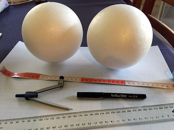
The first physical property of the sun to be measured was how far away it is. In the 3rd century BC, the ancient Greek Aristarchus of Samos (who we met briefly in 2. Eratosthenes’ measurement) developed a method to measure the distance to the sun in terms of the size of the Earth, using the geometry of the relative positions of the sun and moon. Firstly, when the moon appears exactly half-illuminated from a point on Earth, it means that the angle formed by the sun-moon-Earth is 90°. If you observe the angle between the sun and the moon at this time, you can determine the distance to the sun as a multiple of the distance to the moon.

Aristarchus's method 1

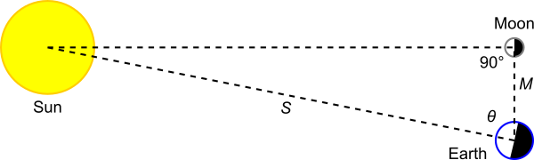
Geometry of the sun, moon, and Earth when the moon appears half-illuminated.

In the figure, if you measure the angle θ, then the ratio of the distance to the sun S divided by the distance to the moon M is the reciprocal of the cosine of θ. Aristarchus then used the size of the shadow of Earth on the moon during a lunar eclipse to obtain further equations relating the distances to the sun and moon and the size of the Earth.

Aristarchus's method 2

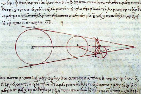
A medieval copy of Aristarchus’s drawing of the geometry of the sun-Earth-moon system during a lunar eclipse. (Public domain image.)

By combining these results, you can calculate the distances to both the sun and the moon in terms of the radius of the Earth. Aristarchus got the wrong answer, estimating that the sun was only about 19 times further away than the moon, because of the limited precision of his naked eye angle measurements (it’s actually 390 times further away). But Eratosthenes later made more accurate measurements (which were again discussed in Eratosthenes’ measurement), most likely using the same method.

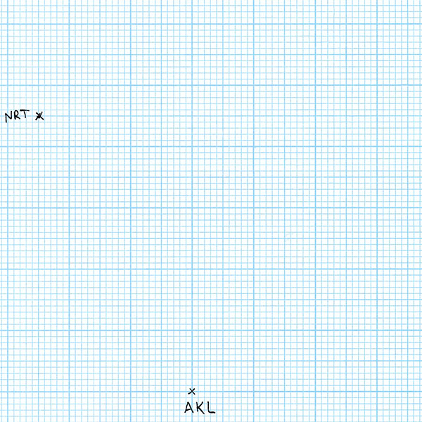
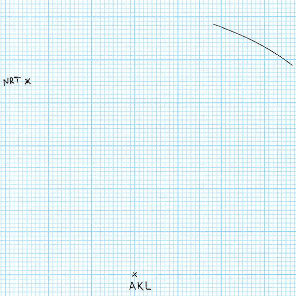
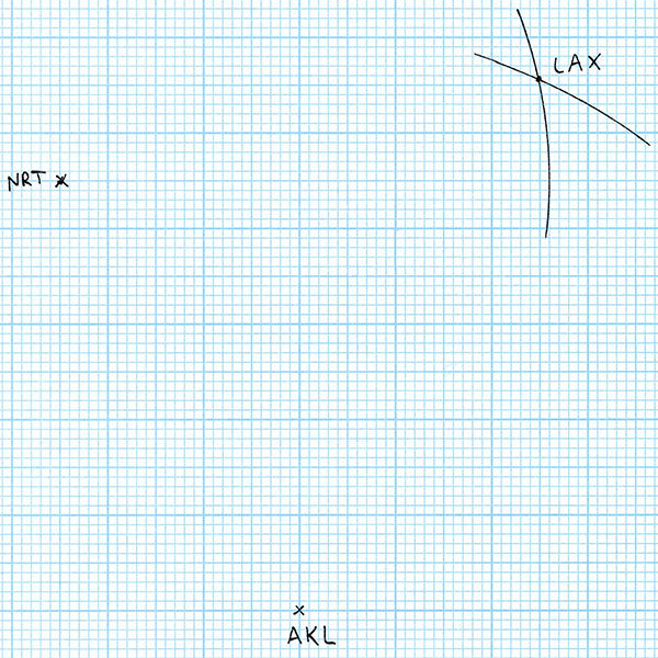
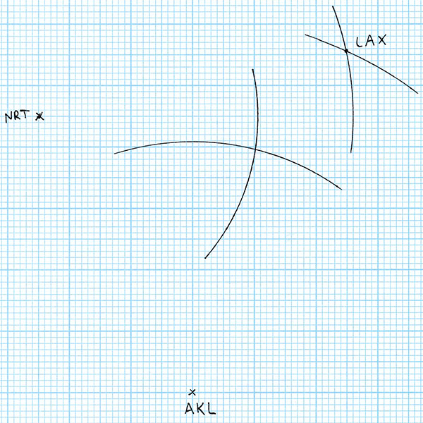
The first rigorous measurement of the absolute distance to the sun was made by Giovanni Cassini in 1672. By this time, observations of all the known celestial bodies in our solar system and some geometry had well and truly established the relative distances of all the orbits. For example, it was known that the orbital radius of Venus was 0.72 times that of Earth, while the orbit of Mars was 1.52 times that of Earth. To measure the absolute distance to the sun, Cassini used a two-step method, the first step of which was measuring the distance to the planet Mars. This is actually a lot easier to do than measuring the distance to the sun, because Mars can be seen at night, against the background of the stars.

Cassini dispatched his colleague Jean Richer to Cayenne in French Guiana, South America, and the two of them arranged to make observations of Mars from there and Paris at the same time. By measuring the angles between Mars and nearby stars, they determined the parallax angle subtended by Mars across the distance between Paris and Cayenne. Simple geometry than gave the distance to Mars in conventional distance units. Then applying this to the relative distances to Mars and the sun gave the absolute distance from the Earth to the sun.

Since 1961, we’ve had a much more direct means of measuring solar system distances. By bouncing radar beams off the moon, Venus, or Mars and measuring the time taken for the signal to return at the speed of light, we can measure the distances to these bodies to high precision (a few hundred metres, although the distances to the planets change rapidly because of orbital motions) [1].

The Earth orbits the sun at a distance of approximately 150 million kilometres. Once we know this, we can work out the size of the sun. The angular size of the sun as seen from Earth can be measured accurately, and is 0.53°. Doing the mathematics, 0.53°×(π/180°)×150 = 1.4, so the sun is about 1.4 million kilometres in diameter, some 109 times the diameter of the Earth. This is the diameter of the visible surface – the sun has a vast “atmosphere” that we cannot see in visible light. Because of its vast distance compared to the size of the Earth, the sun’s angular size does not change appreciably as seen from different parts of the Earth. The difference in angular size between the sun directly overhead and on the horizon (roughly the Earth’s radius, 6370 km, further away) is only about 6370/150000000×(180°/π) = 0.002°.

Our sun is, in fact, a star – a huge sphere composed mostly of hydrogen and helium. It produces energy from mass through well-understood processes of nuclear fusion, and conforms to the observed properties of stars of similar size. The sun appears much larger and brighter than stars, and heats the Earth a lot more than stars, because the other stars are all so much further away.

The Sun

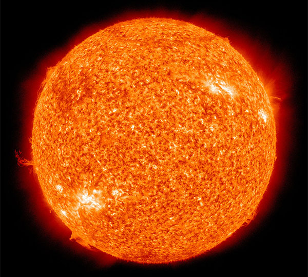
Our sun, observed in the ultraviolet as a false colour image by NASA’s Solar Dynamics Observatory satellite. (Public domain image by NASA.)

Like all normal stars, the sun radiates energy uniformly in all directions. This is expected from the models of its structure, and can be inferred from the uniformity of illumination across its visible disc. The fact that the sun’s polar regions are just as bright as the equatorial edges implies that the radiation we see in the ecliptic plane (the plane of Earth’s orbit) is reproduced in all directions out of the plane as well.

NASA’s Ulysses solar observation spacecraft was launched in 1990 and used a gravity slingshot assist from Jupiter to put it into a solar orbit inclined at about 80° to the ecliptic plane. This allowed it to directly observe the sun’s polar regions.
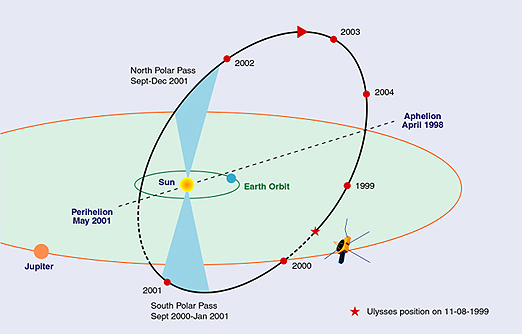
Ulysses' orbit

Polar orbit of Ulysses around the sun, giving it views of both the sun’s north and south poles. (Public Domain image by NASA.)

Now, I tried to find scientific papers using data from Ulysses to confirm that the sun indeed radiates electromagnetic energy (visible light, ultraviolet, etc.) uniformly in all directions. However, it seems that no researchers were willing to dedicate space in a paper to discussing whether the sun radiates in all directions or not. It’s a bit like looking for a research paper that provides data on whether apples fall to the ground or not. What I did find are papers that use data from Ulyssessolar wind particle flux detectors to measure if the energy emitted by the sun as high energy particles varies with direction.

Solar proton flux versus latitude

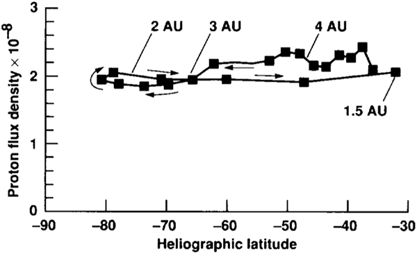
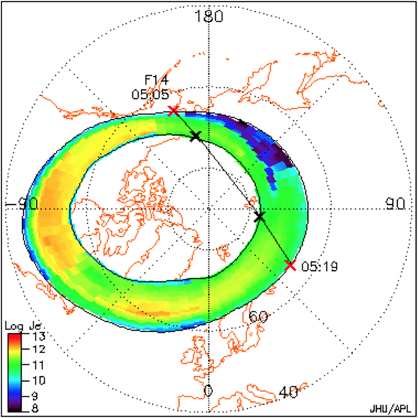
Proton flux density observed by Ulysses at various heliographic (sun-centred) latitudes. -90 is directly south of the sun, 0 would be in the ecliptic plane. The track shows Ulysses’ orbit, changing in distance and latitude as it passes under the sun’s south polar regions. Figure reproduced from [2].

Solar wind energy flux versus latitude

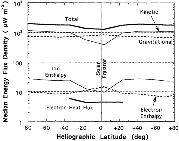
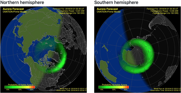
Various solar wind plasma component energy fluxes observed by Ulysses at various heliographic latitudes. Figure reproduced from [3].

As these figures show, the energy emitted by the sun as solar wind particles is pretty constant in all directions, from equatorial to polar. Interestingly, there is a variation in the solar wind energy flux with latitude: the solar wind is slower and less energetic close to the plane of the ecliptic than at higher latitudes. The solar wind, unlike the electromagnetic radiation from the sun, is affected by the structure of the interplanetary medium. The denser interplanetary medium in the plane of the ecliptic slows the wind. The amount of slowing provides important constraints on the physics of how the solar wind particles are accelerated in the first place.

Anyway, given there are papers on the variation of solar wind with direction, you can bet your bottom dollar that there would be hundreds of papers about the variation of electromagnetic radiation with direction, if it had been observed, because it goes completely counter to our understanding of how the sun works. The fact that the sun radiates uniformly in all directions is such a straightforward consequence of our knowledge of physics that it’s not even worth writing a paper confirming it.

Now, in our spherical Earth model, all of the above observations are both consistent and easily explicable. In a Flat Earth model, however, these observations are less easily explained.

Why is the sun visible in the sky from part of the Earth (during daylight hours), while in other parts of the Earth at the same time it is not visible (and is night time)?

The most frequently proposed solution for this is that the sun moves in a circular path above the disc of the Flat Earth, shining downwards with a sort of spotlight effect, so that it only illuminates part of the disc. Although there is a straight line view from areas of night towards the position of the sun in the sky, the sun does not shine in that direction.

Given that we know the sun radiates uniformly in all directions, we know this cannot be so. Furthermore, if the sun were a directional spotlight, how would such a thing even come to be? Directional light sources do occur in nature. They are produced by synchrotron radiation from a rapidly rotating object: for example, a pulsar. But pulsars rotate and sweep their directional beams through space on a timescale of approximately one second. If our sun were producing synchrotron radiation, its spotlight beam would be oscillating many times per minute – something which is not observed.

Even furthermore, if the sun is directional and always above the plane of the Flat Earth, it should be visible in the night sky, as an obscuration passing in front of the stars. This prediction of the Flat Earth model is not seen – it is easy to show that no object the size of the sun obscures any stars at night.

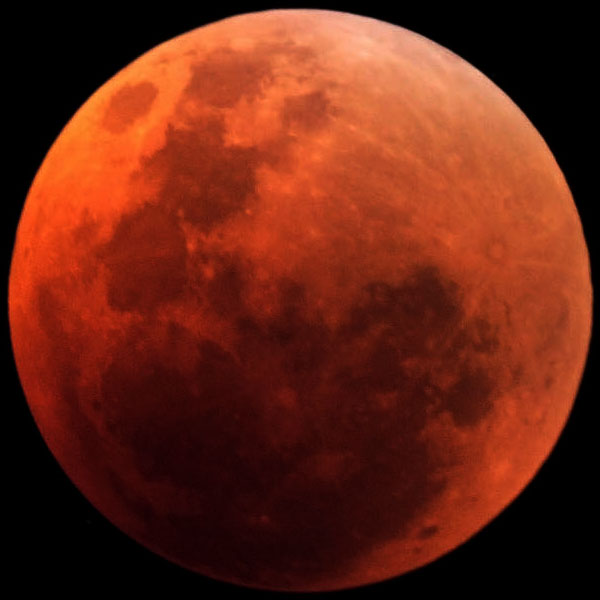
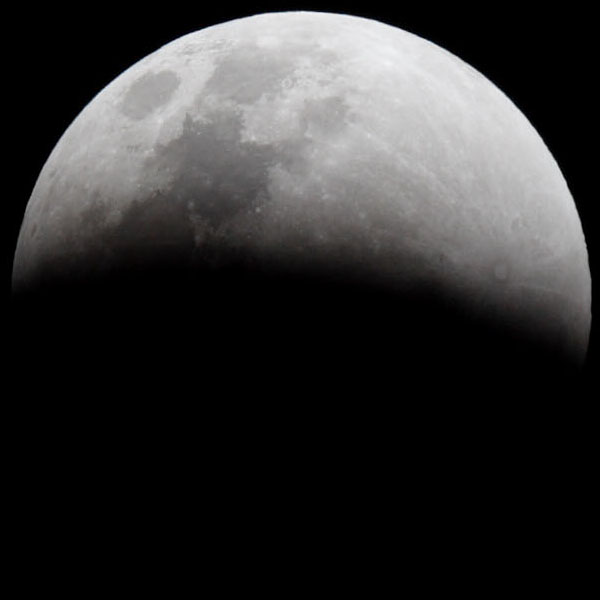
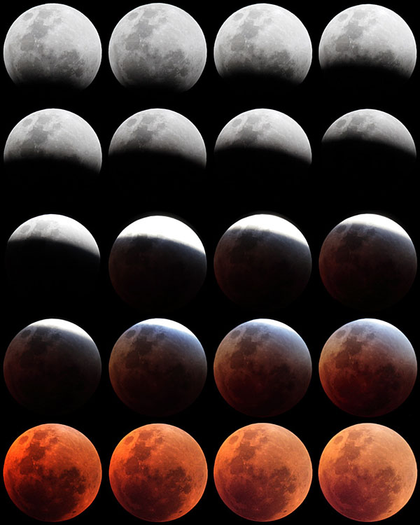
And yet furthermore, if the sun is directional, there are substantial difficulties in having it illuminate the moon. Some Flat Earth models acknowledge this and posit that the moon is self-luminous, and changes in phase are caused by the moon itself, not reflection of sunlight. This can easily be observed not to be the case, since (a) there are dark shadows on the moon caused by the light coming from the location of the sun in space, and (b) the moon darkens dramatically during lunar eclipses, when it is not illuminated by the sun.

In addition to the directional spotlight effect, typical Flat Earth models state that the distance to the sun is significantly less than 150 million kilometres. Flat Earth proponent Wilbur Glenn Voliva used geometry to calculate that the sun must be approximately 3000 miles above the surface of the Earth to reproduce the zenith angles of the sun seen in the sky from the equator and latitudes 45° north and south.

Voliva's distance to the sun calculation

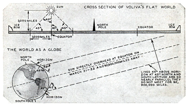
Wilbur Glenn Voliva’s calculation that the sun is 3000 miles above the Flat Earth. Reproduced from Modern Mechanics, October 1931, p. 73.

Aside from the fact that Voliva’s distance does not give the correct zenith angles for any other latitudes, it also implies that the sun is only about 32 miles in diameter, given the angular size seen when it is overhead, and that the angular size of the sun should vary significantly, becoming only 0.53°/sqrt(2) = 0.37° when at a zenith angle of 45°. If the sun is this small, there are no known mechanisms than can supply the energy output it produces. And the prediction that the sun would change in angular size is easily disproved by observation.

The simplest and most consistent way of explaining the physical properties of our sun is in a model in which the Earth is a globe.

References:

[1] Muhleman, D. O., Holdridge, D. B., Block, N. “The astronomical unit determined by radar reflections from Venus”. The Astrophysical Journal, 67, p. 191-203, 1962. https://doi.org/10.1086/108693

[2] Barnes, A., Gazis, P. R., Phillips, J. L. “Constraints on solar wind acceleration mechanisms from Ulysses plasma observations: The first polar pass”. Geophysical Research Letters, 22, p. 3309-3311, 1995. https://doi.org/10.1029/95GL03532

[3] Phillips, J. L., Bame, S. J., Barnes, A., Barraclough, B. L., Feldman, W. C., Goldstein, B. E., Gosling, J. T., Hoogeveen, G. W., McComas, D. J., Neugebauer, M., Suess, S. T. “Ulysses solar wind plasma observations from pole to pole”. Geophysical Research Letters, 22, p. 3301-3304, 1995. https://doi.org/10.1029/95GL03094

11. Auroral ovals

Aurorae are visible light phenomena observed in the night sky, mostly at high latitudes corresponding to Arctic and Antarctic regions. An aurora can appear as an indistinct glow from a distance or as distinct shifting curtain-like formations of light, in various colours, when seen from nearby.

An aurora

An aurora, observed near Eielson Air Force Base, near Fairbanks, Alaska. (Public domain image by Senior Airman Joshua Strang, United States Air Force.)

Aurorae are caused by the impact on Earth’s atmosphere of charged particles streaming from the sun, known as the solar wind.

Solar wind and Earth's magnetosphere

Schematic representation of the solar wind streaming from the sun and interacting with the Earth’s magnetic field. The dashed lines indicate paths of solar particles towards Earth. The solid blue lines show Earth’s magnetic field. (Public domain image by NASA.)

The Earth’s magnetic field captures the particles and deflects them (according to the well-known laws of electromagnetism) so that they spiral downwards around magnetic field lines. The result is that the particles hit the atmosphere near the Earth’s magnetic poles.

Solar wind interacting with Earth's magnetosphere

Diagram of the solar wind interacting with Earth’s magnetic field (field lines in red). The magnetic field deflects the incoming particles around the Earth, except for a fraction of the particles that enter the magnetic polar funnels and spiral down towards Earth’s magnetic poles. (Public domain image by NASA. modified.)

The incoming high energy particles ionise nitrogen atoms in the upper atmosphere, as well as exciting oxygen atoms and nitrogen molecules into high energy states. The recombination of nitrogen and the relaxation of the high energy states results in the emission of photons. The light is produced between about 90 km and 150 km above the surface of the Earth, as shown by triangulating the positions of aurorae from multiple observing locations.

Observations of aurorae have established that they occur in nearly-circular elliptical rings of width equivalent to a few degrees of latitude (i.e. a few hundred kilometres), usually between 10° and 20° from the Earth’s magnetic poles. These rings, in the northern and southern hemispheres, are called the auroral ovals.

Northern auroral oval

Northern auroral oval observed on 22 January 2004. Figure reproduced from [1].

The auroral ovals are not precisely centred on the magnetic poles, but rather are pushed a few degrees towards the Earth’s night side. This is caused by the diurnal deflection of the Earth’s magnetic field by pressure from the charged particles of the solar wind.

Northern auroral oval seen by DE-1

Northern auroral oval observed in 1983 by Dynamics Explorer 1 satellite. The large bright patch at left is the daylight side of Earth. (Public domain image by NASA.)

The auroral ovals also expand when solar activity increases, particularly during solar storms, when increased particle emission from the sun and the resulting stronger solar wind compresses the Earth’s magnetic field, forcing field lines to move away from the poles.

But despite these variations, the auroral ovals in the northern and southern hemispheres move and change sizes more or less in unison, and are always of similar size.

Southern auroral oval

Southern auroral oval observed in 2005 by IMAGE satellite, overlaid on a Blue Marble image of Earth. (Public domain image by NASA.)

You can see the current locations and sizes of both the northern and southern auroral ovals as forecast based on the solar wind and interplanetary magnetic field conditions as measured by the Deep Space Climate Observatory satellite at https://www.spaceweatherlive.com/en/auroral-activity/auroral-oval.

Northern and southern auroral ovals

Current northern and southern auroral ovals as forecast by spaceweatherlive.com on 21 April, 2019. The auroral ovals are the same size and shape.

Earth is not the only planet to display aurorae. Jupiter has a strong magnetic field, which acts to funnel the solar wind towards its polar regions in the same way as Earth’s field does on Earth. Jupiter we can establish by simple observation from ground-based telescopes is close to spherical in shape and not a flat disc. Auroral ovals are observed on Jupiter around both the northern and southern magnetic poles, exactly analogously to on Earth: of close to the same size and shape.

Northern auroral ovals on Jupiter

Auroral ovals on Jupiter observed in the northern and southern polar regions by the Hubble Space Telescope, using the Wide Field Planetary Camera (1996) and the Space Telescope Imaging Spectrograph (1997-2001). Figure reproduced from [2].

Similar auroral ovals are also seen on Saturn, in both the northern and southern hemispheres [3][4]. And just for the record, Saturn is also easily shown to be spherical in shape, and not a flat disc.

Now, we have established that auroral ovals appear on three different planets, with the southern and northern ovals of close to the same sizes and shapes on each individual planet. Everything is consistent and readily understandable – as long as you assume that the Earth is spherical like Jupiter and Saturn.

If the Earth is flat, however, then the distributions of aurorae in the north and south map to very different shapes and sizes – with no ready explanation for either the shapes or their differences. In particular, large parts of the southern auroral oval end up being extremely far from the southern magnetic pole, in defiance of the electromagnetic mechanism that causes aurorae in the first place.

Auroral ovals on a flat Earth

Auroral ovals in their observed locations, mapped onto a flat disc Earth. The ovals are vastly different sizes.

So the positions of aurorae on a flat Earth cannot be readily explained by known laws of physics, and they also do not resemble the locations and sizes of auroral ovals as observed on other planets. All of these problems go away and become self-consistent if the Earth is a globe.

References:

[1] Safargaleev, V., Sergienko, T., Nilsson, H., Kozlovsky, A., Massetti, S., Osipenko1, S., Kotikov, A. “Combined optical, EISCAT and magnetic observations of the omega bands/Ps6 pulsations and an auroral torch in the late morning hours: a case study”. Annales Geophysicae, 23, p. 1821-1838, 2005. https://doi.org/10.5194/angeo-23-1821-2005

[2] Grodent, D.,Clarke, J. T., Kim, J., Waite Jr., J. H., Cowley, S. W. H. “Jupiter’s main auroral oval observed with HST‐STIS”. Journal of Geophysical Research, 108, p. 1389-1404, 2003. https://doi.org/10.1029/2003JA009921

[3] Cowley, S. W. H., Bunce, E. J., Prangé, R. “Saturn’s polar ionospheric flows and their relation to the main auroral oval”. Annales Geophysicae, 22, p.1379-1394, 2004. https://doi.org/10.5194/angeo-22-1379-2004

[4] Nichols, J. D., Clarke, J. T., Cowley, S. W. H., Duval, J., Farmer, A. J., Gérard, J.‐C., Grodent, D., Wannawichian, S. “Oscillation of Saturn’s southern auroral oval”. Journal of Geophysical Research, 113, A11205, 2008. https://doi.org/10.1029/2008JA013444

10. The Sagnac effect

Imagine beams of light coming from an emitter and travelling around a circular path in both directions, until they arrive back at the source. Such an arrangement can be constructed by using an optic fibre in a circular loop, injecting light at both ends. The distance travelled by the clockwise beam is the same as the distance travelled by the anticlockwise beam, and the speed of light in both directions is the same, so the time taken for each beam to travel from the source back to the origin is the same. So far, so good.

A light loop

A loop with light travelling in both directions.

Now imagine the whole thing is rotating – let’s say clockwise. For reference we’ll use the numbers on a clock face and the finer divisions into 60 minutes. The optic fibre ring runs around the edge of the clock, with the light source and a detector at 12. Now imagine that the clock rotates fast enough that by the time the clockwise-going light reaches the original 12 position, the clock has rotated so that 12 is now located at the original 1 minute past 12 position. The light has to travel an extra 60th of the circle to reach its starting position (actually a tiny bit more than that because the clock is still rotating and will have gone a tiny bit further by the time the light beam catches up). But the light going anticlockwise reaches the source early, only needing to travel a tiny bit more than 59/60 of the circle. The travel times of the two beams of light around the circle are different.

A rotating light loop

Now the loop is rotating. By the time the light has travelled around the loop, the exit from the loop has moved a little bit clockwise. So the light travelling clockwise has to travel further to reach the exit, while the light travelling anticlockwise reaches the exit sooner.

This is a very simplified explanation, and figuring out the mathematics of exactly what happens involves using special relativity, since the speed of light is involved, but it can be shown that there is indeed a time difference between the travel times of beams of light heading in opposite directions around a rotating loop. The time difference is proportional to the speed of rotation and to the area of the loop (and to the cosine of the angle between the rotation axis and the perpendicular to the loop, for those who enjoy vector mathematics). This effect is known as the Sagnac effect, named after French physicist Georges Sagnac, who first demonstrated it in 1913.

Measuring the minuscule time difference between the propagation of the light beams is not difficult, due to the wave nature of light itself. The wavelength of visible light is just a few hundred nanometres, so even a time difference of the order of 10-16 seconds can be observed because it moves the wave crests and troughs of the two beams relative to one another, causing visible interference patterns as they shift out of synchronisation. This makes the device an interferometer that is very sensitive to rotational speed.

The Sagnac effect can be seen not only in a circular loop of optic fibre, but also with any closed loop of light beams of any shape, such as can be constructed with a set of mirrors. This was how experimenters demonstrated the effect before the invention of optic fibres. Because the paths of the two beams of light are the same, just reversed, a Sagnac interferometer is completely insensitive to mechanical construction tolerances, and only sensitive to the physical rotation of the device.

Sagnac actually performed the experiment in an attempt to prove the existence of the luminiferous aether, a hypothetical medium permeating all space through which light waves propagate. He believed his results showed that such an aether existed, but Max von Laue and Albert Einstein showed that Sagnac’s effect could be explained by special relativity, without requiring any aether medium for light propagation.

The interesting thing about the Sagnac effect is that it measures absolute rotational speed, that is: rotation relative to an inertial reference frame, in the language of special relativity. In practice, this means rotation relative to the “fixed” position of distant stars. This is useful for inertial guidance systems, such as those found on satellites, modern airliners and military planes, and missiles. The Sagnac effect is used in ring laser gyroscopes and fibre optic gyroscopes to provide an accurate measure of rotational speed in these guidance systems. GPS satellites use these devices to ensure their signals are correctly calibrated for rotation – without them GPS would be less accurate.

Because the magnitude of the Sagnac effect depends on both the rotational speed and the area of the light loop, by making the area large you can make the interferometer incredibly sensitive to even very slow rotation. Rotations as slow as once per 24 hours. You can use these devices to measure the rotation of the Earth.

This was first done in 1925. Albert A. Michelson (of the famous Michelson-Morley experiment that disproved the existence of the luminiferous aether), Henry G. Gale, and Fred Pearson acquired the use of a tract of land in Clearing, Illinois (near Chicago’s Midway Airport), and built a huge Sagnac interferometer, a rectangle 610×340 metres in size [1][2].

Michelson’s Sagnac interferometer

Diagram of Michelson’s Sagnac interferometer in Clearing, Illinois. The Sagnac loop is defined by the mirrors ADEF. The smaller rectangle ABCD was used for calibration measurements. Light enters from the bottom towards the mirror A, which is half-silvered, allowing half the light through to D, and reflecting half in the other direction towards F. The beams complete circuits ADEF and AFED, returning to A, where the half-silvering reflects the beam from D and lets through the beam from F towards the detector situated outside the loop at the left. The light paths are inside a pipe system, which is evacuated using a pump to remove most of the air. (Figure reproduced from [2].)

With this enormous area, the shift in the light beams caused by the rotation speed of the Earth at the latitude of Chicago was around one fifth of a wavelength of the light used – easily observable. The Michelson-Gale-Pearson experiment’s measurements and calculations showed that the rotation speed they measured was consistent with the rotation of the Earth once every 23 hours and 56 minutes – a sidereal day (i.e. Earth’s rotation period relative to the stars; this is shorter than the average of 24 hours rotation relative to the sun, because the Earth also moves around the sun).

Now the interesting thing is that the Sagnac effect measures the linear rotation speed, not the angular rotation rate. The Earth rotates once per day – that angular rotation rate is constant for the entire planet, and can be modelled in a flat Earth model simply by assuming the Earth is a spinning disc, like a vinyl record or Blu-ray disc. But the linear rotation speed of points on the surface of the Earth varies.

In the typical flat Earth model with the North Pole at the centre of the disc, the rotation speed is zero at the North Pole, and increases linearly with distance from the Pole. As you cross the equatorial regions, the rotational speed just keeps increasing linearly, until it is maximal in regions near the “South Pole” (wherever that may be).

Rotation speed on a flat disc Earth

Rotation speeds at different places on a flat rotating disc Earth (top view of the disc).

On a spherical Earth, in contrast, the rotation speed is zero at the North Pole, and varies as the cosine of the latitude as you travel south, until it is a maximum at the equator, then drops again to zero at the South Pole.

Rotation speed on a flat disc Earth

Rotation speeds at different places on a spherical Earth.

Here is a table of rotation speeds for the two models:

Latitude Speed (km/h)
Flat model
Speed (km/h)
Spherical model
90°N (North Pole) 0.0 0.0
60°N 875.3 837.2
41.77°N (Clearing, IL) 1407.2 1248.9
30°N 1750.5 1450.1
0° (Equator) 2625.8 1674.4
30°S 3501.1 1450.1
45.57°S (Christchurch) 3896.6 1213.3
60°S 4376.4 837.2
90°S (South Pole) 5251.6 0.0

In the Michelson-Gale-Pearson experiment, the calculated expected interferometer shift was 0.236±0.002 of a fringe (essentially a wavelength of the light used), and the observed shift was 0.230±0.005 of a fringe. The uncertainty ranges overlap, so the measurement is consistent with the spherical Earth model that they used to calculate the expected result.

If they had used the North-Pole-centred flat Earth model, then the expected shift would have been 1407.2/1248.9 larger, or 0.266±0.002 of a fringe. This is well outside the observed measurement uncertainty range. So we can conclude that Michelson’s original 1925 experiment showed that the rotation of the Earth is inconsistent with the flat Earth model.

Nowadays we have much more than that single data point. Sagnac interferometers are routinely used to measure the rotation speed of the Earth at various geographical locations. In just one published example, a device in Christchurch, New Zealand, at a latitude of 43°34′S, measured the rotation of the Earth equal to the expected value (for a spherical Earth) to within one part in a million [3]. Given that the expected flat Earth model speed is more than 3 times the spherical Earth speed at this latitude—and all of the other rotation speed measurements made all over the Earth consistent with a spherical Earth—we can well and truly say that any rotating disc flat Earth model is ruled out by the Sagnac effect.

References:
[1] Michelson, A. A. “The Effect of the Earth’s Rotation on the Velocity of Light, I.” The Astrophysical Journal, 61, 137-139, 1925. https://doi.org/10.1086%2F142878
[2] Michelson, A. A.; Gale, Henry G. “The Effect of the Earth’s Rotation on the Velocity of Light, II.” The Astrophysical Journal, 61, p. 140-145, 1925. https://doi.org/10.1086%2F142879
[3] Anderson, R.; Bilger, H. R.; Stedman, G. E. “ “Sagnac” effect: A century of Earth‐rotated interferometers”. American Journal of Physics, 62, p. 975-985, 1994. https://doi.org/10.1119/1.17656

9. The South Pole

One of the most popular models for a flat Earth presumes the Earth to be a circular disc centred at the North Pole, and with Antarctica spanning the rim and providing some form of impassable barrier to simply travelling off the disc.

Disc shaped flat Earth

A common Flat Earth model: a flat circular disc centred at the North Pole. (Public domain image from Wikimedia Commons.)

This raises the question of where the South Pole is. In such a disc model, there is no single South Pole – all points on the rim of the disc are equally far south. Yet people have travelled to a single geographic place that matches all of the physical requirements of being the South Pole of a spherical Earth:

1. People heading south always end up at this same spot, no matter which line of longitude they head south along.

2. At this place, the sun circles the horizon once per 24 hour period during the southern hemisphere summer, not setting until the autumn equinox, after which it circles below the horizon throughout the southern winter, only rising again at the spring equinox. This is exactly as expected for a physical South Pole on a spherical planet.

3. The place is directly underneath the point in the sky around which the southern stars appear to revolve, in a manner exactly analogous to the movement of the stars at the North Pole, but in the opposite rotational direction. The stars at the North Pole appear to rotate anticlockwise in the sky, while at the South Pole they rotate clockwise in the sky.

Star trails in the southern hemisphere

Star trails in the southern hemisphere, photographed in the Atacama Desert in Chile. (Creative Commons Attribution 4.0 International image by the European Southern Observatory.) This photo shows the motion of the southern hemisphere stars through several hours of a night, moving in apparent circles around the South Celestial Pole (the point directly above the Earth’s South Pole). I tried to find a copyright or royalty-free photo of star trails photographed from the South Pole itself, but could not find any, however Astronomy Picture of the Day has such a photo taken at the South Pole, showing complete circles over a 24-hour period of darkness.

Furthermore, from this place, or areas around it, there are no directions in which one cannot travel. There is no visible edge of the disc, nor any impassable barrier to travel.

The same argument applies to the North Pole if the flat Earth is supposed to be a disc with the South Pole at its centre. And if the disc is some other configuration, then there will always be some point on the spherical Earth that ends up corresponding to all the points around the rim of the flat disc Earth – where it is straightforward to travel to that point on the spherical Earth but which is unreachable or should display bizarre properties (such as a rim or impassable barrier) on the flat Earth.

All of this is difficult to explain in a flat Earth model, but is a natural consequence of a spherical Earth.

8. Earth’s magnetic field

Magnetic fields have both a strength and a direction at each point in space. The strength is a measure of how strong a force a magnet feels when in the field, and the direction is the direction of the force on a magnetic north pole. North poles of magnets on Earth tend to be pulled towards the Earth’s North Magnetic Pole (which is in fact a magnetic south pole, but called “the North Magnetic Pole” because it is in the northern hemisphere), while south poles are pulled towards the South Magnetic Pole (similarly, actually a magnetic north pole, called “the South Magnetic Pole” because it’s in the south). Humans have used this property of magnets for thousands of years to navigate, with magnetic compasses.

The simplest magnetic field is what’s known as a dipole, because it has two poles: a north pole and a south pole. You can think of this as the magnetic field of a simple bar magnet. The magnetic field lines are loops, with the field direction pointing out of the north pole and into the south pole, and the loops closing inside of the magnet.

A magnetic dipole

Illustration of magnetic field lines around a magnetic dipole. The north and south poles of the magnet are marked.

It’s straightforward to measure both the strength and the direction of the Earth’s magnetic field at any point on the surface, using a device known as a magnetometer. So what does it look like? Here are some contour maps showing the Earth’s magnetic field strength and the inclination – the angle the field lines make to the ground.

Earth's magnetic field intensity

Earth’s magnetic field strength. The minimum field strength occurs over South America; the maximum field strengths occur just off Antarctica, south of Australia, and in the broad patch covering both central Russia and northern Canada. (Public domain image by the US National Ocean and Atmospheric Administration.)

Earth's magnetic field inclination

Earth’s magnetic field inclination. The field direction is parallel to the ground at points along the green line, points into the ground in the red region, and points out of the ground in the blue region. The field emerges vertically at the white mark off the coast of Antarctica, south of Australia – this is the Earth’s South Magnetic Pole. The field points straight down at the North Magnetic Pole, north of Canada – not shown in this Mercator projection map, which omits areas with latitude greater than 70° north or south. (Public domain image by the US National Ocean and Atmospheric Administration.)

Now, how can we explain these observations with either a spherical Earth or flat Earth model? Let’s start with the spherical model.

You may notice a few things about the maps above. The Earth’s magnetic field is not symmetrical at the surface. The lowest intensity point over South America is not mirrored anywhere in the northern hemisphere. And the South Magnetic Pole is at a latitude about 64°S, while the North Magnetic Pole is at latitude 82°N. As it happens, this observed magnetic field is to a first approximation the field of a magnetic dipole – just not a dipole that is centred at the centre of the Earth. The dipole is tilted with respect to Earth’s rotation, and is offset a bit to one side – towards south-east Asia and away from South America. This explains the minimum intensity in South America, and the asymmetry of the magnetic poles.

A magnetic dipole

The Earth’s magnetic field is approximated by a dipole, offset from the centre of the Earth. The rotational axis is the light blue line, with geographic north and south poles marked. The red dots are the equivalent magnetic poles. The North Magnetic Pole is much closer to the geographic north pole than the South Magnetic Pole is to the geographic south pole. (As stated in the text, the “North Magnetic Pole” of the Earth is actually a magnetic south pole, and vice versa.)

Models of the interior of the Earth suggest that there are circulating electrical currents in the molten core, which is composed mostly of iron. These currents are caused by thermal convection, and twisted into helices by the Coriolis force produced by the Earth’s rotation, both well understood physical processes. Circulating electrical currents are exactly what causes magnetic fields. The simplest version of this so-called dynamo theory model is one in which there is a single giant loop of current, generating a simple magnetic dipole. And in fact this dipole fits the Earth’s magnetic field to an average deviation of 16% [1].

This is not a perfect fit, but it’s not too bad. The adjustments needed to better fit Earth’s measured field are relatively small, and can also be understood as the effects of circulating currents in the Earth’s core, causing additional components of the field with smaller magnitudes. (The Earth’s magnetic field also changes over time, but we’ll discuss that another day: Now available in Proof 44. Magnetic striping.)

If the Earth is flat, however, there is no such relatively simple way to understand the strength and direction of Earth’s magnetic field using standard electromagnetic theory. Even the gross overall structure—which is readily explained by a magnetic dipole for the spherical Earth—has no such simple explanation. The shape of the field on a flat Earth would require either multiple electrical dynamos or large deposits of magnetic materials under the Earth’s crust, and they would have to be fortuitously arranged in such a way that they closely mimic a dipole if we assumed the Earth to be a sphere. For any random arrangement of magnetic field-inducing structures on a flat Earth to happen to mimic the field of a spherical planet so closely is highly unlikely. Potentially it could happen, but the Earth actually being a sphere is a much more likely explanation.

That the simpler model is more likely to be true than the one requiring many ad-hoc assumptions is a case of Occam’s razor. In science, particularly, a simpler theory is more easily testable than one with a large number of ad-hoc assumptions. Occam’s razor will come up a lot, and I should probably write a sidebar article about it.

References:

[1] Nevalainen, J.; Usoskin, I.G.; Mishev, A. “Eccentric dipole approximation of the geomagnetic field: Application to cosmic ray computations”. Advances in Space Research, 52, p. 22-29, 2013. https://doi.org/10.1016/j.asr.2013.02.020

7. Supernova 1987A

[audio version of this article]

Stars produce energy from nuclear fusion reactions in their cores, where the light elements making up the bulk of the star are compressed and heated by gravity until they fuse into heavier elements. There is a limit to this, however, because once iron is produced in the core no more energy can be extracted from it. Fusing iron requires an input of energy. As iron accumulates, the layers near the core collapse inwards, because not enough energy is being produced to hold them up. At a certain point, the collapse speeds up suddenly and catastrophically, the whole core of the star collapsing in a few seconds. This releases an enormous amount of gravitational energy, fusing heavier elements and initiating nuclear reactions in the outer parts of the star, which blow off in a vast explosion. The star has turned into a supernova, one of the most energetic phenomena in the universe. A supernova can, briefly, shine brighter than the entire galaxy of 100 billion (1011) stars containing it.

Historically, supernovae were detected visually, when a “new star” suddenly appeared in the night sky, shining brightly for a few weeks before fading away from sight. We have reliable records of visible supernovae appearing in the years 1006, 1054, 1181, 1572, and 1604, as well as unconfirmed but probable events occurring in 185 and 393. These supernovae all occurred within our own Milky Way Galaxy, so were close enough to be visible to the naked eye. Since 1604, there have been no supernovae detected in our Galaxy – which is a bit of a shame because the telescope was invented around 1608, just too late to observe the most recent one.

Astronomers have used telescopes to observe supernovae in other galaxies since the late 19th century. Almost none of these are visible to the naked eye. But in 1987 a supernova occurred in the Large Magellanic Cloud, a dwarf galaxy satellite of our own, making it the nearest supernova ever observed in the telescopic era. It reached magnitude 3, making it as bright as a middling star in our sky. It was first seen by independent observers in Chile and New Zealand on 24 February 1987.

The Large Magellanic Cloud is visible from the southern hemisphere of Earth, and in the north up to a latitude around 21°N. It is never visible from any point further north. And so supernova 1987A (the first supernova detected in 1987) was never visible from any point further north than 21°N.

Supernova 1987A

Supernova 1987A and the Large Magellanic Cloud. SN 1987A is the bright star just right of the centre of the image. (Photo: Creative Commons Attribution 4.0 International by the European Southern Observatory.)

When a supernova explosion occurs, the collapsing star emits vast quantities of matter and radiation into the surrounding space. Visible light is just one part of the radiation. SN 1987A also emitted gamma rays, x-rays, and ultraviolet light, the latter two of which were detected by space-based telescopes. And it also blasted particles into interstellar space: heavy element nuclei, neutrons, electrons, and other subatomic particles. One of the types of particles produced was neutrinos. Neutrinos have such a small mass that so far we’ve been unable to perform any experiment that can distinguish their mass from zero. And this means that they move at close to the speed of light – so close that we’ve never made any observation that shows them to move any slower.

At the moment of collapse, SN 1987A emitted a huge burst of neutrinos. These travelled through intergalactic space and some of the neutrinos made it to Earth, where some of them were detected. This neutrino burst was detected almost simultaneously at three different neutrino observatories in different parts of the world:

While a total of 24 neutrinos might not sound like a lot, this is significantly higher than the background detection rate of neutrinos from other sources such as our sun and general cosmic rays from random directions in space. And all 24 of these neutrinos were detected within a single 13-second time window – if corrected for the differences in light travel time from SN 1987A to each observatory caused by their locations on the spherical Earth.

You might notice that all three of the detectors listed are in the northern hemisphere. In fact, the southernmost of them is Kamioka, at 36° 20′ 24″ N. This means that the Large Magellanic Cloud, and SN 1987A in particular, are not visible in the sky at any of these detector locations. This fact by itself provides fairly convincing evidence to most people that the Earth cannot be flat, but Flat Earth enthusiasts propose various solutions for the limited visibility of celestial objects from different parts of the Earth. In Flat Earth theory, all visible stars and galaxies are above the plane of the Earth, and obscured from some parts by distance or intervening objects. This obviously requires SN 1987A to be above the plane of the Flat Earth.

In fact, at this point it might seem that the spherical Earth has a problem: If SN 1987A is not visible from the locations of the neutrino detectors, then how did they detect neutrinos from it? The answer is that neutrinos are extremely elusive particles – they barely interact with matter at all. Neutrinos are known to pass right through the Earth with ease. So although the spherical Earth blocked the light from SN 1987A from reaching the neutrino observatories, it did not stop the neutrinos. The neutrinos passed through the Earth to reach the observatories.

Astronomers estimate SN 1987A released around 1058 neutrinos. The blast was 168,000 light years away, so at the distance of Earth, the number of neutrinos passing through the Earth would be approximately 3×10²⁰ neutrinos per square metre. The Kamiokande-II detector is a cylinder of water 16 metres high and 15.6 metres in diameter, so nearly 1023 SN 1987A neutrinos would have passed through it, leading to just 11 detections. This matches the expected detection rate for neutrinos very well.

Additionally, the Kamioka and Irvine-Michigan-Brookhaven detectors are directional – they can determine the direction from which observed neutrinos arrive. They arrived coming up from underground, not down from the sky. The observed directions at both detectors correspond to the position of the Large Magellanic Cloud and SN1987A on the far side of the spherical Earth [1][2].

Kamiokande-II results

Distribution of SN 1987A neutrino detections at Kamiokande-II in energy of produced electrons and angle relative to the direction of the Large Magellanic Cloud (LMC). Detected electrons are produced by two different processes, the first is rapid and highly aligned with neutrino direction, while the second is a slower secondary particle generation process and randomises direction uniformly. Neutrinos 1 and 2 (the earliest in the burst) are aligned directly with the LMC, and the remainder are distributed uniformly. This is statistically consistent with the burst having originated from the LMC. Figure reproduced from [1].

In a flat Earth model, SN 1987A would have to be simultaneously above the plane of the Earth (to be visible from the southern hemisphere) and below it (for the neutrino burst to be visible coming up from under the plane of the Earth). This is self-contradictory. However the observations of SN 1987A are all consistent with the Earth being a globe.

References:

[1] Hirata, K.; Kajita, T.; Koshiba, M.; Nakahata, M.; Oyama, Y.; Sato, N.; Suzuki, A.; Takita, M.; Totsuka, Y.; Kifune, T.; Suda, T.; Takahashi, K.; Tanimori, T.; Miyano, K.; Yamada, M.; Beier, E. W.; Feldscher, L. R.; Kim, S. B.; Mann, A. K.; Newcomer, F. M.; Van, R.; Zhang, W.; Cortez, B. G. “Observation of a neutrino burst from the supernova SN1987A”. Physical Review Letters, 58, p. 1490-1493, 1987. https://doi.org/10.1103/PhysRevLett.58.1490

[2] Bratton, C. B.; Casper, D.; Ciocio, A.; Claus, R.; Crouch, M.; Dye, S. T.; Errede, S.; Gajewski, W.; Goldhaber, M.; Haines, T. J.; Jones, T. W.; Kielczewska, D.; Kropp, W. R.; Learned, J. G.; Losecco, J. M.; Matthews, J.; Miller, R.; Mudan, M.; Price, L. R.; Reines, F.; Schultz, J.; Seidel, S.; Sinclair, D.; Sobel, H. W.; Stone, J. L.; Sulak, L.; Svoboda, R.; Thornton, G.; van der Velde, J. C. “Angular distribution of events from SN1987A”. Physical Review D, 37, p. 3361-3363, 1988. https://doi.org/10.1103/PhysRevD.37.3361