Category: Proof

The earliest method of marking time during the day was by following the movements of the sun as it crossed the sky, from sunrise in the east to sunset in the west. The apparent motion of the sun makes the shadows of fixed objects move during the day too. If you poke a stick into the ground, the shadow of the stick moves across the ground as time passes. By making marks on the ground and seeing which one the shadow is near, you get a method of telling the time of day. This is a simple form of sundial.

The apparent motion of the sun in the sky is caused by the interaction between the Earth’s orbit around the sun and the rotation of the Earth on its axis, which is inclined at approximately 23.5° to the axis of the orbital plane. At the June solstice (roughly 21 June), the northern hemisphere is maximally pointed towards the sun, making it summer while the southern hemisphere has winter. Half a year later at the December solstice, the sun is on the other side of the Earth, making it summer in the south and winter in the north. Midway between the solstices, at the March and September equinoxes, both hemispheres receive the same amount of sun.

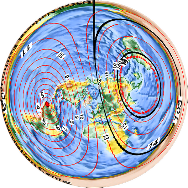
From the point of view of an observer standing on the Earth’s surface, the motions of the Earth make it appear as though the sun moves across the sky once per day, and drifts slowly north and south throughout the year. The following diagram shows the path of the sun across the sky for different dates, for my home of Sydney (latitude 34°S).

In the diagram, the horizon is around the edge, and the centre of the circles is directly overhead. The blue lines show the sun’s path for the indicated dates of the year. The sun is lowest in the sky to the north, and visible for the shortest time, on the June solstice (the southern winter), while it is highest in the sky and visible for the longest on the December solstice (in summer). The red lines show the position of the sun along each arc at the labelled hour of the day. For a location in the northern hemisphere north of the tropics, the sun paths would be curved the other way, passing south of overhead. In the tropics (between the Tropics of Capricorn and Cancer), some paths are to the north while some are to the south. On the equinoxes (20 March and 21 September), the sun rises due east at 06:00 and sets due west at 18:00 – this is true for every latitude.

If you have a fixed object cast a shadow, that shadow moves throughout the course of a day. The next day, if the sun has moved north or south because of the slowly changing seasons, the path the shadow traces moves a little bit above or below the previous day’s path.

The ancient Babylonians and Egyptians used sundials, and the ancient Greeks used their knowledge of geometry to develop several different styles. Greek sundials typically used a point-like object, called the nodus, as the reference marker. The nodus could be the very tip of a stick, a small ball or disc supported by thin wires, or a small hole that lets a spot of sunlight through. The shadow of the nodus (or the spot of light in the case of a hole nodus) moves across a surface in a regular way, not just with time of day, but also with the day of the year. During the day, the point-like shadow of a nodus traces a path from west to east (as the sun moves east to west in the sky). Throughout the year, the daily path moves north and south as the sun moves further south or north in the sky due to the seasons.

There are two slight complications. The red lines in the sun’s path diagram show timing of the sun paths assuming the Earth’s orbit is perfectly circular, but in reality it is an ellipse, with the Earth nearest the sun in January and furthest away in June. Earth travels around that elliptical path at different speeds—due to Newton’s law of gravity and laws of motion—moving fastest at closest approach in January, and slowest in June. The result of this is that the daily interval between when the sun crosses the north-south line is 24 hours on average, but varies systematically through the year. This variation in the sun’s apparent motion has a period of one year.

The second complication occurs because of the tilt of the Earth’s axis to the ecliptic plane in which it orbits. The sun’s apparent movement in the sky is due west (parallel to the Earth’s equator) only at the equinoxes. On any other date it moves at an angle, with a component of motion north or south, as it moves up or down the sky with the seasons. This north-south motion is maximal at the solstices. So at the solstices the westward component of the sun’s motion is less than it is at the equinoxes, meaning that it appears to move westward across the sky more slowly (because part of its speed is being used to move north or south). This variation in the sun’s apparent motion has a period of half a year.

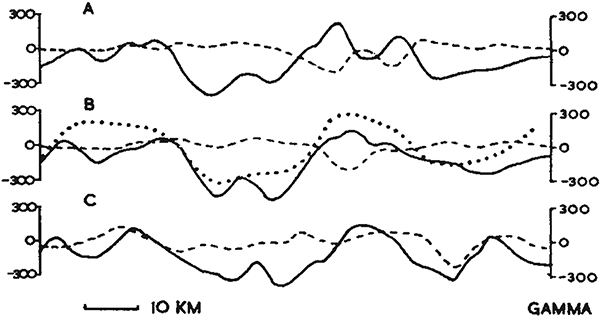
To get the total variation in the sun’s motion, we need to add these two components. Doing so gives us the equation of time. This is the amount of time by which the sun’s position varies from the ideal “circular orbit, non-inclined axial spin” case, as a function of the day of the year.

What this means is that if you have a standard sort of simple sundial, the shadow moves at different speeds across the face on different dates of the year, resulting in the shadow getting a little bit ahead or a little bit behind clock time. To get the correct time as shown by a clock, you need to read the time off the sundial’s shadow and subtract the number of minutes given by the equation of time for that date.

But this is thinking about sundials with our modern mindest about how time works. We have decided to make the unit of time we call a “day” the average length of time that it takes the sun to return to its highest position in the sky, and then we’ve divided that day into 24 exactly equal hours. An hour on 20 March is exactly the same length as an hour on 21 June, or on 21 December. “Of course it is!” you say.

But it wasn’t always so. For most of history, a “day” was defined as either the time between one sunrise and the next, or one sunset and the next, or the time between when the sun was due south in the sky and when it returned to being due south again (in the northern hemisphere). Each of these definitions of a “day” vary in length throughout the year. Saudi Arabia officially used Arabic time up until 1968, which defined midnight (the start of a new day) to be at sunset each day, and clocks needed to be adjusted every day to track the shift in sunset through the seasons.

The definition of a day as the period between the sun being due south (or north) and returning to that position the next day, is called solar time. For most of human timekeeping history, this is what was used. The fact that some days were a bit longer or shorter than others was of no consequence when the sun itself was the best timekeeping tool that anyone had access to.

Our modern concept of an hour has its origins in ancient Egypt, around 2,500 BC. The Egyptians originally divided the night time period into 12 parts, marked by the rising of particular stars in the sky. Because the stars change with the seasons (as discussed in 36. The visible stars), they had tables of which stars marked which hours for different dates of the year. Because of precession of the Earth’s orbit, the stars fell out of synch with the tables over the course of several centuries.

The oldest non-sundial timekeeping device that still exists is a water clock dating from the reign of Amenhotep III, around 1350 BC. It was a conical bowl, which was filled with water at sunset, and had a small outflow drip hole that let water out at a roughly constant rate. Inside the bowl is a set of 12 level marks, showing the water level at each of the 12 divisions of the night. But not just one set of 12 marks – there are multiple sets of 12 markings, with different spacings, that show the passage of the night time hours for different months of the year, when the length of the night is different.

The oldest sundial we have is also from ancient Egypt, dating from around 1500 BC, a piece of limestone with a hole bored in it for a stick, and shadow marks, 12 of them, for dividing the daylight hours into 12 parts.

So the ancient Egyptians were dividing both the daylight and night time parts of each day into 12 different-length parts for a total of 24 divisions. Through cultural contact, sundials became a common way to mark the 12 hours of daylight in many other Mediterranean and Middle Eastern civilisations too, including the ancient Greeks and Romans.

By the Middle Ages, Catholic Europe was still keeping time based on a division of daylight time into 12 variable-length hours, and this carried across to the canonical hours, marking the times of day for liturgical prayers:

• Matins: the night time prayer, recited some time after midnight, but before dawn.
• Lauds: the dawn prayer, taking place at first light.
• Prime: recited during the first hour of daylight.
• Terce: at the third hour of the day time.
• Sext: at midday, at the sixth hour, when the sun is due south.
• Nones: the ninth hour of the day time.
• Vespers: the sunset prayer, at the twelfth hour of the daylight period.
• Compline: the end of the working day prayer, just before bed time.

In the modern world we might interpret “the third hour” to be 9:00 am, halfway between 6:00 am and midday, but the canonical hours are guided by the sun, so Terce would be earlier in summer and later in winter, in the same way that sunrise, and hence the celebration of Lauds, are. Nones, in contrast, would be earlier in winter and later in summer. (Incidentally, we get our modern word “noon” from “Nones” – although you’ll notice that Nones was defined as the ninth hour, or around 3:00 pm. For some reason it moved to become associated with the middle of the day. We’re not sure exactly why, but historians believe that the monks who observed this liturgy fasted each day until after the prayer of Nones, so there was constant pressure to make it slightly earlier, which eventually moved it back a full three hours!)

You might think that when mechanical clocks were invented, people suddenly realised that they’d been doing things wrong the whole time, and they quickly moved to the modern system of an hour being of a constant length. But that’s not what happened. The first mechanical clocks used a verge escapement to regulate the motion of the gear wheels, and this remained the most accurate clock mechanism from the 13th century to the 17th. But it wasn’t very accurate, varying by around 15 minutes per day, and so verge clocks had to be reset daily to match the motion of the sun.

Christiaan Huygens invented the pendulum clock in 1656, vastly improving the accuracy of mechanical clocks, down to around 15 seconds per day. With this new level of accuracy, people fully realised for the first time that the length of a full day as measured by the time it took the sun to return to the highest position in the sky didn’t match a regularly ticking clock. But rather than adjust their definition of what an hour was, people decided there must be a way to get these regular clocks to tell proper solar time! Thus were invented equation clocks.

The first equation clocks had a correction dial, which essentially displayed the equation of time value for the current day of the year. You read the time off the main clock dial, and then added the correction displayed on the correction dial, and that gave you the “correct” solar time. By the 18th century, the correction gearing was incorporated into the main clock face display, so that the hands of the clock actually ran faster or slower at different times of the year, to match the movement of the sun. It wasn’t until the early 19th century that European society moved to a mean time system (“mean” as in “average”), in which each “day” was defined to be exactly the same length, and the hour was a fixed period of time (thus simplifying clockmakers’ lives considerably).

Just to complete this story, clocks in the early 19th century were set to local mean time, which was the mean time of their meridian of longitude. Towns a few tens of miles east or west would have different mean times by a few minutes. This caused problems beginning with the introduction of rapid travel enabled by the railways, eventually leading to the adoption of standard time zones in the 1880s, in which all locations in slices of roughly 1/24 of the Earth share the same time.

What this means is that people were still living their lives by local solar time up until the early 19th century. In other words, a sundial was still the most accurate method of telling the time up until just 200 years ago – and it didn’t need any corrections based on the equation of time because people weren’t using mean time yet. It’s only in the past 200 years that we’ve had to correct a sundial to give what we consider to be the correct clock time.

So, back to sundials. Assuming we are happy with solar time (and can use the equation of time to correct to mean time if we wish), the main thing we need to contend with is that the sun moves north and south in the sky throughout the year. A nodus-type sundial accounts for this by marking lines that indicate the time when the shadow of the nodus crosses them on different days of the year. But many sundials use the whole edge of a stick or post as the shadow marker – this edge is called the gnomon. As the sun moves north and south throughout the year, different parts of the gnomon will cast their shadows in different places. If the gnomon is aligned parallel to the axis of the Earth, then these motions will be along the edge of the shadow, rather shifting the edge of the shadow laterally. You can then read solar time using a single marking, at any time of the year.

Another way to think about it is that from a viewpoint on Earth, the sun appears to revolve in the sky about the Earth’s axis. So if your sundial has a gnomon that is parallel to the Earth’s axis, the sun appears to rotate with the gnomon as its axis once per day, and the shadow of the gnomon indicates solar time on the marked surface below. As the sun moves north or south with the seasons, it is still revolving around the gnomon, so the shadow still tracks solar time accurately. If the gnomon is not parallel to the revolution axis, then as the sun moves north and south, the shadow of the gnomon will shift positions on the marked surface, and the time will be inaccurate at different times of the year.

This is why sundials with gnomons all have them inclined at an angle from the horizontal equal to the latitude of where the sundial is placed. At the North Pole, a vertical stick will indicate solar time accurately throughout the entire summer (when the sun is above the horizon 24 hours a day). At London (latitude 51.5°N), sundial gnomons are pointed north at 51.5° from the horizontal.

At Perth, Australia (32°S), they point south and are 32° from the horizontal, noticeably flatter.

A sundial on the equator must have a gnomon that is horizontal.

So, in order to work properly, gnomon-sundials must have a gnomon angled parallel to the Earth’s axis of rotation. The fact that sundials at different latitudes need to have their gnomons at different angles to the ground plane shows that the ground plane is only perpendicular to the Earth’s rotation axis at the North and South Poles, and the angle between the ground and Earth’s axis of rotation varies everywhere else in a way consistent with the Earth being a globe.

If the Earth were flat… well, all of this would just be a huge coincidence in the motion of the sun above the flat Earth, that for some unexplained reason exactly mimics the geometry of a spherical Earth in orbit about the sun. In fact, to get all of the angles to match sundial observations you need to posit that the sun’s rays don’t even travel in straight lines.

Addendum: I just wanted to show you this magnificent sundial, in the Monastery of Lluc, in Mallorca, Spain.

This sundial has five separate faces:

Top left shows the canonical hours. At sunrise (no matter what time sunrise happens to be), the shadow of the stick indicates the liturgy of Prime. Sext occurs at solar noon, when the sun is directly overhead, with Terce halfway between Prime and Sext. Vespers is at sunset (again, regardless of the modern clock time), with Nones halfway between Sext and Vespers. The night time hours of Complice, Matins, and Lauds are marked above the horizontal (and in fact would correctly indicate the times if the Earth were transparent, so the sun could cast a shadow from underneath the horizon).

Bottom left shows a nodus sundial, the tip of the stick marking “Babylonian” hours, which were used in Mallorca historically. This counts 0 (or 24) at sunrise, and then equal numbered hours thereafter. The vertical position of the nodus shadow marks the date (similar to the Krakow sundial above).

The central dial is a gnomon indicating “true solar time”. The shadow of the edge of the gnomon indicates the solar hour.

Finally the two dials on the right are nodus dials, showing mean time horizontally, and date of the year vertically. The top dial is to be read in summer and autumn, whole the lower dial is for winter and spring. It looks like the dials also include a daylight saving adjustment, assuming it begins and ends on the equinoxes!

The time (confirmed from the photo EXIF data) is 4:15 pm, and the date is 9 September, 12 days before the autumnal equinox (read on the top right dial).

References:

[1] “Polar sun path chart program”, University of Oregon Solar Radiation Monitoring Laboratory. http://solardat.uoregon.edu/PolarSunChartProgram.html

[2] Ritner, Robert. “Oriental Institute Museum Notes 16: Two Egyptian Clepsydrae (OIM E16875 and A7125)”. Journal of Near Eastern Studies, 75, p. 361-389, 2016. https://doi.org/10.1086/687296

References:

[1] Yaplee, B. S., Bruton, R. H., Craig, K. J., Roman., N. G. “Radar echoes from the moon at a wavelength of 10 cm.” Proceedings of the Institute of Radio Engineers, 46(1), p. 293-297, 1958. https://doi.org/10.1109/JRPROC.1958.286790
[2] Yaplee, B. S., Knowles, S. H., Shapiro, A., Craig, K. J., Brouwer, D. “The mean distance to the Moon as determined by radar.” In Symposium-International Astronomical Union, 21, p. 81-93, Cambridge University Press, 1965. https://doi.org/10.1017/S0074180900104826
44. Magnetic striping
We’ve discussed continental drift and plate tectonics in Proof 22. Plate tectonics. There’s another aspect of plate tectonics that was mentioned in passing there, which deserves some further attention. Proof 22 stated:
But as technology advanced, detailed measurements of the sea floor were made beginning in the late 1940s, including the structures, rock types, and importantly the magnetic properties of the rocks.
That last one, the “magnetic properties”, was the piece of evidence that really cemented continental drift as a real thing.
We pick up the history in 1947, when research expeditions led by American oceanographer Maurice Ewing established the existence of a long ridge running roughly north-south down the middle of the Atlantic Ocean. They also found that the crust beneath the ocean was thinner than that beneath the continents, and that the rocks (below the seafloor sediment) were basalts, rather than the granites predominantly found on continents. There was something peculiar about the Earth’s crust around these mid-ocean ridges. And over the next few years, more ridges were found in other oceans, revealing a network of the structures around the globe. The system of mid-ocean ridges had been discovered, but nobody yet had an explanation for it.
Meanwhile, from 1957, the Russian-American oceanographer Victor Vacquier took World War II surplus aerial magnetometers that had been used to detect submerged submarines from reconnaissance aircraft, and adapted them for use in submarines to examine the magnetic properties of the sea floor. It was well known that basalt contained the mineral magnetite, which is rich in iron and can be strongly magnetised.
What Vacquier found was unexpected and astonishing. In a survey of the Mendocino Fault area off the coast of San Francisco, Vacquier discovered that the sea floor basalt was not uniformly magnetised, but rather showed a distinctive and striking pattern. The magnetism appeared to be relatively constant along north-south lines, but to vary rapidly along the east-west direction, causing “stripes” of magnetism running north-south.[1]
Magnetic field measurements on the sea floor near Mendocino Fault
Map of magnetic field measurements on the sea floor near Mendocino Fault, showing strong north-south striping of the magnetic field. (Figure reproduced from [1].)
Follow up observations showed that the stripes were not localised, but extended over large regions of the ocean.[2][3].
Magnetic anomalies on the sea floor off California
Map of magnetic anomalies on the sea floor off California. Shaded areas are positive magnetic anomaly, unshaded areas are negative. (Figure reproduced from [2].)
In fact, these magnetic “zebra stripes” were present pretty much everywhere on the floor of every ocean. They weren’t always aligned north-south though – it turned out that they were aligned parallel to the mid-ocean ridges. The early discoverers of this odd phenomenon had no explanation for it.
Returning to the mid-ocean ridges, American oceanographer Bruce Heezen wrote a popular article in Scientific American in 1960 that informed readers of the recent discoveries of these enormous submarine geological features.[4] In the article, he speculated that perhaps the ridges were regions of upwelling material from deep within the Earth, and the sea floors were expanding outwards from the ridges. Heezen was not aware of any mechanism for regions of Earth’s crust to disappear, so he suggested that the Earth might slowly be expanding, through the creation of new crust at the mid-ocean ridges.
Although Heezen’s idea of an expanding Earth didn’t take hold, his idea of upwelling and expansion along the mid-ocean ridges was quickly combined with existing proposals (that Heezen had overlooked) that crust could be disappearing along the lines of deep ocean trenches, as parts of the Earth moved together and were subducted downwards. The American geologists Harry Hammond Hess and Robert S. Dietz independently synthesised the ideas into a coherent theory of continental drift, combining the hypotheses of seafloor spreading and ocean trench subduction to conclude that the Earth was not changing size, but rather it was fractured into crustal plates that slowly moved, spreading apart in some places, and colliding and subducting in others.[5][6]
Proposed mantle convection by Hess
Earliest diagrams of proposed mantle convection cells causing continental drift, with upwelling at mid-ocean ridges causing seafloor spreading, by Harry Hammond Hess. Figure 7 (top) shows the detailed structure of a mid-ocean ridge, with measured seismic velocities (the speed of seismic waves in the rock) in various regions. Hess proposed that the observed lower speeds in the central and upper zones were caused by fracturing of the rock as it deforms during the upwelling, plus higher residual temperature of the upwelled material. Figure 8 (bottom) shows Hess’s proposed mantle convection cells. (Figures reproduced from [6].)
So by the 1960s, most of the observational pieces of this puzzle were in place. However, the unifying theory that would explain it all still required some synthesis, and acceptance of some unestablished hypotheses. This synthesis was again put together independently by two different groups of geologists: the Canadian Lawrence Morley, and the English Ph.D. student Frederick Vine and his supervisor Drummond Matthews. Morley wrote two papers and submitted them to Nature and the Journal of Geophysical Research in 1963, but both journals rejected his work as too speculative. Vine and Matthews thus received publication priority when Nature accepted their paper later in 1963.[7]
The geologists pointed out that if new rock was being created at the mid-ocean ridges and then spreading outwards, then the seafloor rocks should get progressively older the further away they are from the ridges. Each one of the magnetic zebra stripes running parallel to the ridges then corresponds to rocks of the same age. If, they conjectured, the rocks record the direction of the Earth’s magnetic field when they were formed, and for some reason the Earth’s magnetic field reversed direction periodically, that would explain the existence of the magnetic stripes.
Observed and modelled sea floor magnetic fields
Diagram by Vine and Matthews showing the observed magnetic field strength of the sea floor rocks measured across the Carlsberg Ridge in the Indian Ocean, showing positive and negative regions (solid lines), computed magnetic field strength under conventional (for the time) assumptions (dashed lines), and computed field strength assuming 20 km wide bands in which the Earth’s magnetic field has been reversed. The periodic field reversal matches the observed magnetism much better. (Figure reproduced from [7].)
As with Morley’s rejected papers, this paper was treated with scepticism initially, because it relied on two unproven conjectures: (1) that the rocks maintain magnetism aligned with the Earth;’s magnetic field at the time of solidification and, much more unbelievably, (2) that the Earth’s magnetic field direction reverses periodically. For some geologists, this was too speculative to be believe.
One test of Vine and Matthews’ seafloor spreading hypothesis would be to measure the age of the sea floor using some independent method. If the rocks were found to get progressively older the further away they are from the mid-ocean ridges, then that would be strong evidence in favour of the theory. As it happens, it’s possible to date the age of rocks formed from magma, using a method of radiometric dating known as potassium-argon (K-Ar) dating. Potassium is a fairly common element in rocks, and the isotope potassium-40 is radioactive, with a half-life of 1.248×10⁹ years. Most of the potassium-40 decays to calcium-40 via beta decay (see Proof 29. Neutrino beams for a recap on beta decay), but just over 10% of it decays via electron capture to the inert gas argon-40. Argon is not present in newly solidified rock, but the argon produced by decaying potassium-40 is trapped within the crystal structure. Since the decay rate is known very precisely, we can use the measured ratio of potassium to argon in the rock to determine how long it has been since it formed, for timescales from several million to billions of years.
In the mid-1960s, oceanographers and geologists began drilling cores and taking basalt samples from the sea floor and measuring their ages.[8] And what they found matched the prediction from seafloor spreading: the youngest rocks were at the ridges and became progressively older towards the edges of the oceans.
Age of oceanic crust
Diagram of the age of oceanic crust. The youngest rocks are red, and found along the mid-ocean ridges. Rocks are progressively older further away from the ridges. (Figure reproduced from [9].)
This was exactly what Vine and Matthews predicted. Belatedly, Morley also received his due credit for coming up with the same idea, and their proposal is now known as the Vine-Matthews-Morley hypothesis. The magnetic striping of the ocean floors is caused by the combination of the spreading of the ocean floors from the mid-ocean ridges, and the periodic reversal of Earth’s magnetic field.
Generation of magnetic striping
Generation of magnetic striping on the sea floor. As the sea floor spreads, and the Earth’s magnetic field reverses from time to time, stripes of different magnetic polarity are created and spread outwards. (Public domain image by the United States Geological Survey, from Wikimedia Commons.)
Odd reversals of magnetic fields in continental rocks had been noticed since 1906, when the French geologist Bernard Brunhes found that some volcanic rocks were magnetised in the opposite direction to the Earth’s magnetic field. In the 1920s, the Japanese geophysicist Motonori Matuyama noticed that all of the reversed rocks found by Brunhes and others since were older than the early Pleistocene epoch, around 750,000 years ago. He suggested that the Earth’s field may have changed direction around that time, but his proposal was largely ignored.
With the impetus provided by the seafloor spreading idea, geologists began measuring magnetic fields and ages of more rocks, and found that they matched up with the ages of the field reversals implied by the sea floor measurements. Progress was rapid and the geological community turned around and developed and adopted the whole theory of plate tectonics within just a few years. By the end of the 1960s, what had been ridiculed less than a decade earlier was mainstream, brought to that status by the confluence of multiple lines of observational evidence.
It had been established that the Earth’s magnetic field must reverse direction with periods of a few tens of thousands to millions of years. The remaining question was how?
Up until the development of plate tectonics, the origin of the Earth’s magnetic field had been a mystery. Albert Einstein even weighed in, suggesting that it might be caused by an imbalance in electrical charge between electrons and protons. But plate tectonics not only raised the question – it also suggested the answer.
The core of the Earth was known to be mostly metallic (see Proof 43. The Schiehallion experiment). If there are convection currents in the mantle, then heat differentials at the boundary should also cause convection within the core. The convecting metal induces electrical currents, which in turn produce a magnetic field. In short, the core of the Earth is an electrical dynamo. And because the outer core is liquid, the currents are unstable. Modern computer simulations of convection in the Earth’s core readily produce instabilities that act to flip the polarity of the magnetic field at irregular intervals – exactly as observed in the record of magnetic striped sea floor rocks.
Simulations of magnetic field reversal in Earth's core
Computer simulations of convection currents in the Earth’s core and resulting magnetic field lines. Blue indicates north magnetic polarity, yellow south. The left image indicates Earth in a stable state, with a magnetic north pole at the top and a south at the bottom. The middle image is during an instability, with north and south intermingled and chaotic. The right image is after the unstable period, with the north and south poles now flipped. (Public domain images by NASA, from Wikimedia Commons.)
So we have a fully coherent and self-consistent theory that explains the observations of magnetic striping, along with many other features of the Earth’s geophysics. It involves several interlocking components: convection in the metallic core producing electric currents that generate a magnetic field that is unstable over millions of years and flips polarity at irregular intervals; convection in the mantle producing upwellings of material along mid-ocean ridges, leading to seafloor spreading and continental drift; rocks that record both their age and the direction and strength of the Earth’s magnetic field when they are formed, leading to magnetic striping on the ocean beds.
Of course, this only holds together and makes sense on a spherical Earth. We’ve already seen in Proof 8. Earth’s magnetic field, that simply generating the shape of the planet’s magnetic field only works on a spherical Earth, and is an inexplicable mystery on a flat Earth model. It would be even more difficult to explain the irregular reversal of polarity of the magnetic field without a spherical core dynamo system. And plate tectonics just doesn’t work on a flat Earth either (Proof 22. Plate tectonics). Combining the fact that neither of these explanations work on a flat Earth, there is no explanation for the observed magnetic striping of the sea floors either. So magnetic striping provides another proof that the Earth is a globe.
[1] Vacquier, V., Raff, A.D., Warren, R.E. “Horizontal displacements in the floor of the northeastern Pacific Ocean”. Geological Society of America Bulletin, 72(8), p.1251-1258, 1961. https://doi.org/10.1130/0016-7606(1961)72[1251:HDITFO]2.0.CO;2
[2] Mason, R.G. Raff, A.D. “Magnetic survey off the west coast of North America, 32 N. latitude to 42 N. Latitude”. Geological Society of America Bulletin, 72(8), p.1259-1265, 1961. https://doi.org/10.1130/0016-7606(1961)72[1259:MSOTWC]2.0.CO;2
[3] Raff, A.D. Mason, R.G. “Magnetic survey off the west coast of North America, 40 N. latitude to 52 N. Latitude”. Geological Society of America Bulletin, 72(8), p.1267-1270, 1961. https://doi.org/10.1130/0016-7606(1961)72[1267:MSOTWC]2.0.CO;2
[4] Heezen, B.C. “The rift in the ocean floor”. Scientific American, 203(4), p.98-114, 1960. https://www.jstor.org/stable/24940661
[5] Dietz, R.S. “Continent and ocean basin evolution by spreading of the sea floor”. Nature, 190(4779), p.854-857, 1961. https://doi.org/10.1038%2F190854a0
[6] Hess, H.H. “History of Ocean Basins: Geological Society of America Bulletin”. Petrologic Studies: A Volume to Honour AF Buddington, p.559-620, 1962. https://doi.org/10.1130/Petrologic.1962.599
[7] Vine, F.J. Matthews, D.H. “Magnetic anomalies over oceanic ridges”. Nature, 199(4897), p.947-949, 1963. https://doi.org/10.1038/199947a0
[8] Orowan, E., Ewing, M., Le Pichon, X. Langseth, M.G. “Age of the ocean floor”. Science, 154(3747), p.413-416, 1966. https://doi.org/10.1126/science.154.3747.413
[9] Müller, R.D., Sdrolias, M., Gaina, C. Roest, W.R. “Age, spreading rates, and spreading asymmetry of the world’s ocean crust”. Geochemistry, Geophysics, Geosystems, 9(4), 2008. https://doi.org/10.1029/2007GC001743
43. The Schiehallion experiment
The Ancients had the technology and cleverness to work out the shape of the Earth and its diameter (see 2. Eratosthenes’ measurement). However, they had no reliable method to measure the mass of the Earth, or equivalently its density, which gives the mass once you know the volume. You could assume that the Earth has a density similar to rock throughout, but there was no way of knowing if that was correct.
In fact we had no measurement of the density or mass of the Earth until the 18th century. Perhaps surprisingly, there wasn’t even any observational evidence to decide whether the Earth was actually a solid object, or a hollow shell with a relatively thin solid crust. As late as 1692 the prominent scientist Edmond Halley proposed that the Earth might be composed of a spherical shell around 800 km thick, with two smaller shells inside it and a solid core, all separated by a “luminous” atmosphere (which could escape and cause the aurora borealis).
Edmond Halley's hollow Earth model
Structure of the Earth as proposed by Edmond Halley in 1692, with solid shells (brown) separated by a luminous atmosphere, shown in cross section.
In his 1687 publication of Philosophiæ Naturalis Principia Mathematica, Isaac Newton presented his theory of universal gravitation. Although this provided explicit equations relating the physical properties of gravitational force, mass, and size, for the cases of astronomical objects there were still more than one unknown value, so the equations could not be solved to determine the absolute masses or densities of planets. The best astronomers could do was determine ratios of densities of one planet to another.
But Newton not only proposed his formulation of gravity as a theoretical construct – he also suggested a possible experiment that could be done to test it. As observed by common experience, objects near the surface of the Earth fall downwards – they are attracted towards the centre of the Earth (more precisely, the Earth’s centre of mass). But if the attractive force of gravity is generated by mass as per Newton’s formulation, then unusual concentrations of mass should change the direction of the gravitational pull a little.
We’ve already seen in Proof 24. “Gravitational acceleration variation” that the strength of Earth’s gravitational pull varies across the Earth’s surface due to differences in altitude and density within the Earth. Now imagine a large concentration of mass on the surface of the Earth. If Newton is correct, then such a mass should pull things towards it. The attraction to the centre of the Earth is much stronger, so the direction of the overall gravitational pull should still be almost downwards, but there should be a slight deflection towards the large mass.
There are some convenient large masses on the surface of the Earth. We call them mountains. Newton conceived that one could go somewhere near a large mountain and measure the difference in angle between a plumb line (which indicates the direction of gravity, and is commonly called “vertical”) and a line pointing towards the Earth’s centre of mass (which does not have a well-defined name, since it is more difficult to measure and differs from a plumb line by an amount too small to be significant in engineering or construction – for the purposes of this proof only, I shall abbreviate it to “downwards”). However, Newton believed that any such difference would be too small to measure in practice. He writes in the Principia, Book 3: On the system of the world:
Hence a sphere of one foot in diameter, and of a like nature to the earth, would attract a small body placed near its surface with a force 20,000,000 times less than the earth would do if placed near its surface; but so small a force could produce no sensible effect. If two such spheres were distant but by 1/4 of an inch, they would not, even in spaces void of resistance, come together by the force of their mutual attraction in less than a month’s time; and lesser spheres will come together at a rate yet slower, namely in the proportion of their diameters. Nay, whole mountains will not be sufficient to produce any sensible effect. A mountain of an hemispherical figure, three miles high, and six broad, will not, by its attraction, draw the pendulum two minutes out of the true perpendicular; and it is only in the great bodies of the planets that these forces are to be perceived.[1]
Here is where Newton’s lack of experience as an experimentalist let him down. Two minutes of arc was already within the accuracies of stellar positions claimed by Tycho Brahe some 80 years earlier. If Newton had merely asked astronomers if they could measure a deflection of such a small size, they would likely have answered yes.
Tycho Brahe in his observatory at Uraniborg
Engraving of Tycho Brahe observing in his observatory at Uraniborg, Sweden. (Public domain image from Wikimedia Commons.)
If you can measure how big the deflection angle is with sufficient accuracy, then you can use that measurement to calculate the density of the Earth in terms of the density of the mountain:
ρE/ρM = (VM/VE) (rE/d)2 / tan θ
where:
ρE is the density of the Earth,
ρM is the density of the mountain,
VE is the volume of the Earth,
VM is the volume of the mountain,
rE is the radius of the Earth,
d is the horizontal distance from the centre of the mountain to the plumb bob, and
θ is the angle of deflection of the plumb line from “downwards”.
The volume of the mountain can be estimated from its size and shape, and the density may be assumed to be that of common types of rock. All the other values were known, leaving the as yet unknown density of the Earth as a function of the deflection angle.
Two French astronomers, Pierre Bouguer (who we met in 4. Airy’s coal pit experiment) and Charles Marie de La Condamine, were the first to attempt to make the measurement. In 1735 they led an expedition to South America to measure the length of an arc of one degree of latitude along a line of longitude near the equator. This was part of an experiment by the French Academy of Sciences—along with simultaneous expedition to Lapland to make a similar measurement near the North Pole—to measure the shape of the Earth. Not whether it was spherical; any difference between the measurements would show if it was more accurately a prolate or an oblate ellipsoid.
Bouguer and La Condamine spent ten years on their expedition, making many other physical, geographical, biological, and ethnographical studies. One experiment they tried in 1738 was measuring the deflection of a plumb bob near the 6263 metre high volcano Chimborazo, in modern day Ecuador.
Chimborazo in Ecuador
The volcano Chimborazo in Ecuador. (Creative Commons Attribution 2.0 image by David Ceballos, from Flickr.)
They climbed to an altitude of 4680 m on one flank of the mountain and 4340 m on the other side, battling harsh weather to take the two measurements. Taking two measurements on opposite sides of the mountain allows a subtraction to remove sources of error in locating the “downwards” direction, leaving behind the difference in angle between the two plumb bob directions, which is twice the desired deflection. Bouguer and La Condamine measured a deflection of 8 seconds of arc, however they considered the circumstances so difficult as to render it unreliable. But they did state that this measurement gave a large value for the Earth’s density, thus disproving the hypothesis that the Earth was hollow.
A more precise measurement of the gravitational deflection of a mountain had to wait until 1772, when Astronomer Royal Nevil Maskelyne made a proposal to repeat the experiment to the Royal Society of London.[2] The Society approved, and appointed the quaintly named Committee of Attraction to ponder the proposal. The committee (counting Joseph Banks and Benjamin Franklin among its members) despatched astronomer and surveyor Charles Mason (of Mason-Dixon line fame) to find a suitable mountain. He came back with Schiehallion, a 1083 m peak in central Scotland.
Schiehallion in Scotland
Schiehallion in central Scotland. (Creative Commons Attribution 3.0 Unported image by Wikipedia user Andrew2606, from Wikimedia Commons.)
Schiehallion had several advantages for the measurement. It’s conveniently located for a British expedition. It’s an isolated peak, with no other mountains nearby that could substantially complicate the effects of gravity in the region. It has a very symmetrical shape, making it easy to estimate the volume with some accuracy. And the northern and southern slopes are very steep, which means that by doing the experiment on those sides, the plumb bob can be positioned relatively close to the centre of mass of the mountain, increasing the deflection and making it easier to measure.
Maskelyne himself led the expedition, taking temporary leave from his post as Astronomer Royal. The party built temporary observatories on the northern and southern flanks of Schiehallion, from which they made frequent observations of overhead stars to determine the zenith line (marking the “downwards” direction), so they could compare it to the direction of the hanging plumb line. Maskelyne and his team spent 6 weeks at the southern observatory, followed by 10.5 weeks at the northern one, battling inclement weather to take the required number of observations.[3]
Map of Schiehallion and surrounds
Map of Schiehallion and surrounds. The mountain forms a short ridge running approximately east-west. The positions of the north and south observatories can be seen. (Reproduced from [6].)
Maskelyne had calculated that if the Earth as a whole had the same density as the mountain (i.e. that of quartzite rock), then they should have observed a deflection of the plumb line relative to “downwards” of 20.9 seconds of arc. Preliminary calculations showed a deflection of about half that, meaning the Earth was roughly twice as dense as the mountain.
To mark the successful conclusion of the observations, the expedition celebrated with a rollicking good party. Plenty of alcohol was imbibed (quite possibly Scotch whisky). In the revelry, unfortunately someone accidentally set fire to the northern observatory and it burnt to the ground. The fire claimed the violin of one Duncan Robertson, a junior member of the expedition who had helped to pass the long cold nights of observation by entertaining the other members with his playing. Later, a grateful Maskelyne sent Robertson a replacement violin – not just any violin, but one made by the master craftsman Antonio Stradivari.[4][5]
The mathematician and surveyor Charles Hutton was charged with doing the detailed calculations of the result. He published them in a mammoth 100-page paper in 1778.[6] His final conclusion was that the density of the Earth was 1.8 times the density of the quartzite in Schiehallion, or about 4.5 g/cm3. Since this was so much higher than the densities of various types of rock (typically between 2 and 3 g/cm3), Hutton concluded (correctly) that much of the core of the Earth must be metal, and he calculated that about 65% of the Earth’s diameter must be a metallic core (a little higher than current measurements of 55%).
Hutton's conclusions on the structure of Earth and density of planets
Extract of Hutton’s paper, where he states that roughly 2/3 of the diameter of the Earth must be metallic to account for the measured density. This page also shows Hutton’s calculations of the densities of solar system bodies. (Reproduced from [6].)
This was the very first time that we had any estimate of the density/mass of the Earth, and Hutton also used it to calculate the densities of the Sun, the Moon, and the planets (out to Saturn) based on their known astronomical properties, mostly to within about 20% of the modern values. So the Schiehallion experiment was groundbreaking and significantly increased our fundamental understanding of the Earth and the solar system.
Later experiments confirmed the general nature of the result and refined the figures for the density and structure of the Earth. In particular, Henry Cavendish—a chemist who 20 years earlier had discovered the elemental nature of hydrogen and made several other discoveries about air and elemental gases—turned his attention to physics and performed what has become known as the Cavendish experiment in 1797-98. He constructed a finely balanced mechanism with which he could measure the tiny gravitational attractive force between two balls of lead, which allowed the measurement of the (then unknown) value of Newton’s gravitational constant. Knowing this value, it becomes possible to directly plug in values for the size of the Earth and the acceleration due to gravity and determine the mass of the Earth. Cavendish’s result was accurate to about 1%, confirming Hutton’s conclusion that the Earth must have a core denser than rock. And then in the 20th century, seismology allowed us to confirm the existence of discrete layers within the Earth, with the central core made primarily of metal (a story for a future Proof).
Drawing of Henry Cavendish
Drawing of Henry Cavendish. (Creative Commons Attribution 4.0 International image by the Wellcome Collection of the British Library, from Wikimedia Commons.)
Of course, the conclusions of the Schiehallion experiment—consistent with later experiments using independent methods—depend on the fact that the Earth is very close to spherical, and the fact that gravity works as Newton said (disregarding the later refinement by Einstein, which is not significant here). One of the more popular Flat Earth models assumes that gravity does not even exist as a force, and that objects “fall” to Earth because the Flat Earth is actually accelerating upwards. In such a model, objects always fall directly “downwards” and there is no deflection caused by large masses such as mountains. The Schiehallion experiment directly and simply disproves this Flat Earth model.
If we suppose that a Flat Earth somehow manages to exist with Newtonian gravity (in itself virtually impossible, see 13. Hydrostatic equilibrium), we could posit something like the 859 km thick flat disc mentioned in 34. Earth’s internal heat. Firstly, Newtonian gravity on such a disc would not always pull perpendicular to the ground – inhabitants near the circumference would be pulled at a substantial angle towards the centre of the disc. Ignoring this, if you managed to do the Schiehallion experiment (say at the North Pole), the distance rE in the equation would be effectively 430 km (the distance to the centre of mass of the disc) rather than the radius of the spherical Earth, 6378 km. This should make the observed deflection angle approximately (6378/430)2 = 220 times smaller! Then the observed deflections would imply that the density of the Earth is 220 times higher, or around 990 g/cm3, about 6 times as dense as the core of the Sun. Which is then inconsistent with the assumed density being the same as the spherical Earth (among other problems).
On the other hand, if we allow the density to be a free parameter, we can solve the gravitational and geometric equations simultaneously to derive the thickness of the Flat Earth disc in a “consistent” manner. This produces a thickness of 3020 km, and a density of 92 g/cm3. Which is over 4 times as dense as osmium, the densest substance at non-stellar pressures. So we’ve shown that the Schiehallion experiment proves that this “Newtonian Flat Earth” model cannot possibly be composed of any known material.
Basically, the observations of the Schiehallion experiment cannot be made consistent with a flat Earth, thus providing evidence that the Earth is a globe.
[1] Newton, I. Philosophiae Naturalis Principia Mathematica (1687). Trans. Andrew Motte, 1729.
[2] Maskelyne, N. “A proposal for measuring the attraction of some hill in this Kingdom”. Philosophical Transactions of the Royal Society, 65, p. 495-499, 1772. https://doi.org/10.1098/rstl.1775.0049
[3]. Sillitto, R.M. “Maskelyne on Schiehallion: A Lecture to The Royal Philosophical Society of Glasgow”. 1990. http://www.sillittopages.co.uk/schie/schie90.html
[4] Davies, R. D. “A Commemoration of Maskelyne at Schiehallion”. Quarterly Journal of the Royal Astronomical Society, 26, p. 289, 1985. https://ui.adsabs.harvard.edu/abs/1985QJRAS..26..289D
[5] Danson, E. Weighing the World. Oxford University Press, 2005. ISBN 978-0-19-518169-2.
[6] Hutton, C. “An Account of the Calculations made from the Survey and Measures taken at Schehallien, in order to ascertain the mean Density of the Earth”. Philosophical Transactions of the Royal Society. 68, p. 689-788, 1778. https://doi.org/10.1098/rstl.1778.0034
42. Schumann resonances
A waveguide is a structure that restricts the motion of waves, disallowing propagation in certain directions, and thus concentrating the energy of the wave to propagate in specific other directions. An example of a waveguide is an optical fibre, which is basically a long, thin string of flexible glass or transparent polymer. Light entering one end is channelled along the fibre, unable to escape from the sides, and emerges at almost the same brightness from the far end.
Normally light and other electromagnetic waves, as well as other waves such as sound, spread out in three dimensions. As the energy spreads out to cover more space, conservation of energy causes the power to fall off according to the inverse square law: power falls as the reciprocal of the square of the distance from the source.
With a waveguide, propagation of the wave can be restricted to a single dimension so the energy doesn’t spread out, resulting in all of the energy being transmitted to the far end (minus a small fraction that may be absorbed or otherwise lost along the way). Sound waves, for example, can be guided by simple hollow tubes, the sound preferring to propagate along the interior air channel than penetrate the tube walls. This is the principle behind medical stethoscopes and old fashioned speaking tube systems.
Another type of waveguide is a transmission line, which is a pair of electrical cables used to transmit alternating current (AC) electrical power. The cables can simply be parallel wires in close proximity, or a coaxial cable, in which an insulated wire runs down the core of tubular conductor. Domestic AC power has a frequency of 50 to 60 hertz, which is low compared to the kilohertz range of radio frequencies. Transmission lines can carry electromagnetic waves up to frequencies of around 30 kHz. Above this, paired wires start to radiate radio waves, so they become inefficient and a different type of waveguide is used.
Radio waveguides are commonly hollow metal tubes. Radio waves travel along the tube, and the conductive metal prevents the waves from leaking to the outside. Such waveguides are used to transmit radio power in radar systems and microwaves in microwave ovens. Anywhere there is a cavity bounded by regions that waves cannot pass through, a waveguide effect can be generated.
A microwave waveguide
A microwave waveguide, which is essentially a hollow metal tube, but precisely machined to optimal dimensions and with high precision connector joints. (Creative Commons Attribution 2.0 image by Oak Ridge National Laboratory, from Flickr.)
Radio waves travel easily through the Earth’s atmosphere, to and from transmission towers and the various wireless devices we use. However the bulk of the Earth is opaque to radio waves; you generally need a mostly unobstructed line of sight, barring relatively thin obstructions like walls.
But there is another region of the Earth that is opaque to (at least some) radio waves. The ionosphere is the region of the atmosphere in which incoming solar radiation ionises the atmospheric gases (mentioned previously in 31. Earth’s atmosphere). It lies between approximately 60 to 1000 km altitude. Since ionised gas conducts electricity, low frequency radio waves cannot pass through it (higher frequencies oscillate too rapidly for the ionised particles to respond).
Opacity of atmosphere vs wavelength
Opacity of the Earth’s atmosphere as a function of electromagnetic wavelength. Long wavelength (low frequency) radio waves are blocked by the ionosphere (right). Other parts of the electromagnetic spectrum are blocked by other aspects of the atmosphere. (Modified from a public domain image by NASA, from Wikimedia Commons.)
Radio waves with wavelengths longer than about 30 metres—or frequencies below about 10 MHz—are thus trapped in the atmosphere between the Earth’s surface and the ionosphere. This forms a waveguide which can carry so-called shortwave radio signals around the world, alternately bouncing off the ionosphere and the Earth’s surface.
There are also natural sources of low frequency radio waves. Lightning flashes in storm systems produce huge discharges of electrical energy, and the sudden release of this energy generates radio waves. If you’ve ever listened to a radio during a thunderstorm you’ll be familiar with the bursts of static caused by strokes of lightning. Lightning generates broadband radio emissions, meaning it covers a wide range of radio frequencies, including the very low frequencies that are guided by the ionospheric waveguide.
Atmospheric scientists measure the amount of lightning around the world by monitoring tiny changes in the Earth’s magnetic field, of the order of picoteslas, caused as these radio waves pass by. The sensitive detectors they use can detect lighting strikes anywhere on the planet. There are a few specific radio frequencies at which the lightning strikes turn out to be especially strong. The following plot shows the intensity of magnetic field fluctuations as a function of radio frequency.
Measurements of magnetic field fluctuation amplitude vs radio frequency
Measurements of magnetic field fluctuation amplitude versus radio wave frequency, averaged over a year of observation, at Maitri Research Station, Antarctica. (Figure reproduced from [1].)
The first peak in the observed radio spectrum is at 7.8 Hz, followed by peaks at 14.3 Hz, 20.8 Hz, and roughly every 6.5 Hz thereafter. People familiar with wave theory will recognise from the pattern that these are likely resonance frequencies, with a fundamental mode at 7.8 Hz, followed by overtones. A wave resonance occurs when an exact number of wavelengths fits into a confined cavity. The wave propagates and bounces around and, because of the precise match with the cavity size, reflected waves end up with peaks and troughs in the same physical position, reinforcing one another. So at the specific resonance frequency, the wave builds up in intensity, while at other frequencies the waves self-interfere and rapidly die down. These resonance frequencies, which are measured at many research stations around the world, are known as Schumann resonances.
The Irish physicist George Francis FitzGerald first anticipated the existence of Schumann resonances in 1893, but his work was not widely circulated. Around 1950, the German physicist Winfried Otto Schumann performed the theoretical calculations that predicted the resonances may be observable, and made efforts to observe them. But it was not until 1960 that Balser and Wagner made the first successful observations and measurements of Schumann resonances.[2]
What causes the radio waves produced by lightning flashes to have a resonance at 7.8 Hz? Well, radio waves travel at the speed of light, so let’s divide the speed of light by 7.8 to see what the wavelength is: the answer is 38,460 km. If you’ve been paying attention to many of these articles, you’ll realise that this is very close to the circumference of the Earth.
Radio waves with a frequency of 7.8 Hz are travelling around the world in the waveguide formed by the Earth and the ionosphere, and returning one wavelength later to constructively interfere and reinforce themselves, producing a measurable peak in Earth’s magnetic field fluctuations at 7.8 Hz. The resonance peak is broad and a little different to 7.5 Hz (the speed of light divided by the circumference of the Earth) because the geometry of a spherical cavity is more complicated than a simple circular loop – effectively some propagation paths are shorter because the waves don’t all take a great circle route.
Schumann resonances diagram
Illustration of Schumann resonances in the Earth’s atmosphere. The ionosphere keeps low frequency radio waves confined to a channel between it and the Earth. Waves propagate around the Earth. At specific frequencies the peaks and troughs line up, producing a resonance that reinforces those frequencies. The blue wave fits six wavelengths around the Earth, the red wave fits three. The fundamental frequency Schuman resonance of 7.8 Hz fits one wave. Not to scale: the ionosphere is much closer to the surface in reality. (Public domain image by NASA/Simoes.)
So Schumann resonances are an observed phenomenon that has a natural explanation – if the Earth is a globe.
If the Earth were flat, then any ionosphere above it would be flat as well, and would still form a waveguide for low frequency radio waves. However it would not be a closed waveguide. Radio waves would propagate out the edges and be lost to space, meaning there would be no observable magnetic field resonances at all. And even if there were an opaque radio wall of some sort at the edge of the flat Earth, the size and geometry of the resulting cavity would be different, resulting in a different set of resonance frequencies, more akin to the frequencies of a vibrating disc, which are not evenly spaced like the observed Schumann resonances.
And so Schumann resonances provide another proof that the Earth is a globe.
[1] Shanmugam, M. “Investigation of Near Earth Space Environment”. Ph.D. Thesis, Manonmaniam Sundaranar University, 2016. https://www.researchgate.net/publication/309209580_Investigation_of_Near_Earth_Space_Environment
[2] Balser, M., Wagner, C. “Observations of Earth–Ionosphere Cavity Resonances”. Nature, 188, p. 638-641, 1960. https://doi.org/10.1038/188638a0
41. Cosmic rays
The French physicist Henri Becquerel discovered the phenomenon of radioactivity in 1896, while performing experiments on phosphorescence – the unrelated phenomenon that causes “glow in the dark” materials to glow for several minutes after being exposed to light. He was interested to see if phosphorescence was related to x-rays, discovered only a few months earlier by Wilhelm Roentgen. In his experiments, Becquerel noticed that uranium salts could darken photographic film, even if wrapped in black paper so that no light could fall on the film, and even from non-phosphorescent uranium samples. The conclusion was that some sort of penetrating rays were being emitted by the uranium itself, without being excited by external energy.
Henri Becquerel in his lab width=
Henri Becquerel in his lab. (Public domain image from Wikimedia Commons.)
Marie and Pierre Curie quickly discovered other radioactive elements, and Becquerel himself discovered by experimenting with magnets that there were three different types of radioactive radiation: two deflected in different directions by a magnetic field and one not deflected at all. In 1899, Ernest Rutherford characterised the first two types, naming them alpha and beta particles, with positive and negative electric charges. Becquerel measured the mass/charge ratio of beta particles in 1900 and determined that they were the same as the electrons discovered by J. J. Thomson in 1897. In 1907 Rutherford showed that alpha particles were the nuclei of helium atoms. And in 1914, he showed that the third type of radiation, named gamma rays, were a form of electromagnetic radiation.
Ernest Rutherford with Hans Geiger
Ernest Rutherford (right), in his lab with Hans Geiger (left), inventor of the Geiger counter. (Public domain image from Wikimedia Commons.)
This was an exciting time in physics, and our understanding of atomic structure was revolutionised within the space of two decades. Besides discovering the basic structure of the atom and how it related to the phenomenon of radioactive decay, several peripheral phenomena also came to the attention of scientists.
One observation was that atoms in the atmosphere were sometimes ionised, or “electrified” as the scientists of the time described it. Ionisation is the process of electrons being stripped off neutral atoms, to form negatively charged free electrons and positively charged atomic ions (consisting of the atomic nucleus and a less-than-full complement of electrons). It was clear that radioactive rays could ionise atoms in the air, and so scientists assumed that it was radiation from radioactive elements in the ground that was ionising the air near ground level.
Father Theodor Wulf
Except strangely the amount of ionising radiation in the atmosphere seemed to increase with increasing altitude. German physicist and Jesuit priest Theodor Wulf invented in 1909 a portable electroscope capable of measuring the ionisation of the atmosphere. He used it to investigate the source of the ionising radiation by measuring ionisation at the base and the top of the Eiffel Tower. He found that the ionisation at the top of the 300 metre tower was a bit over half that at ground level, which was higher than he expected, since theoretically he expected the ionisation to drop by half every 80 metres, so to be less than one tenth the ionisation at ground level. He concluded that there must be some other source of ionising radiation coming from above the atmosphere. However, his published paper was largely ignored.
In 1911, the Italian physicist Domenico Pacini measured the ionisation rates in various places, including mountains, lakes, seas, and underwater. He showed that the rate dropped significantly underwater, and concluded that the main source of radiation could not be the Earth itself. Then in 1912, Austrian physicist Victor Hess took some Wulf electroscopes up in a hot air balloon to altitudes as high as 5300 metres, flying both in daylight, night time, and during an almost complete solar eclipse.
Victor Hess in a hot air balloon flight
Victor Hess (centre), after one of his balloon flight experiments. (Public domain image from Wikimedia Commons.)
Hess showed that the amount of ionising radiation decreased as one moved from ground level up to about 1000 metres, but then increased again rapidly. At 5300 metres, there was approximately twice as much ionising radiation as at ground level.[1] And because the effect occurred at night, and during a solar eclipse, it wasn’t due to the sun. Hess had proven that there was a source of this radiation outside the Earth’s atmosphere. Further unmanned balloon flights as high as 9 km showed the radiation increased even higher with altitude.
Atmospheric radiation readings recorded by Victor Hess
Readings of ionising radiation level (columns 2 to 4) at different altitudes (column 1, in metres), as recorded by Victor Hess. (Figure reproduced from [1].)
What this mysterious radiation was remained unknown until the late 1920s. It was initially thought to be electromagnetic radiation (i.e. gamma rays and x-rays). Robert Millikan named them cosmic rays in 1925 after proving that they originated outside the Earth. Then in 1927 the Dutch physicist Jacob Clay performed measurements while sailing from Java to the Netherlands, which showed that their intensity increased as one moved from the tropics to mid-latitudes.[2] He correctly deduced that the intensity was affected by the Earth’s magnetic field, which implied the cosmic rays must be charged particles.
Atmospheric radiation readings recorded by Jacob Clay
Data recorded by Jacob Clay showing change in ionising radiation with latitude during his voyage from Java to Europe. (Figure reproduced from [2].)
In 1930, the Italian Bruno Rossi realised that if cosmic rays are electrically charged, then they should be deflected either east or west by the Earth’s magnetic field, depending on whether they are positively or negatively charged, respectively.[3] Experiments found that at all locations on the Earth’s surface there are more cosmic rays coming from the west than from the east, showing that most (if not all) cosmic ray particles are positively charged. This observation was called the east-west effect.
Illustration showing incoming cosmic rays deflected to the east
Illustration of the east-west effect. In the space around the Earth (shown as black in this diagram), the Earth’s magnetic field is directed perpendicularly out of the diagram. Incoming cosmic rays are shown in red. When they encounter Earth’s magnetic field, charged particles are deflected perpendicular to the field direction. Positively charged particles are deflected to the right, as shown, meaning that from the surface of the Earth, cosmic rays tend to preferentially come from the west.
Subsequent experiments determined that around 90% of cosmic rays entering our atmosphere are protons, 9% are helium nuclei (or alpha particles), and the remaining 1% are nuclei of heavier elements, with an extremely small number of other types of particles. And in 1936, for his crucial part in the discovery in cosmic rays, Victor Hess was awarded the Nobel Prize for Physics.
The origin of cosmic rays is however still not entirely clear. Our sun produces energetic particles that reach Earth, but cosmic rays are generally defined as coming from outside our own solar system. Our Milky Way Galaxy produces some of the lower energy particles, mostly from the direction of the galactic core, however at very high energies there is a deficit of cosmic rays in that direction, implying a shadowing effect on rays whose origin lies outside our galaxy. Known sources of cosmic rays include supernova explosions, supernova remnants (such as the Crab Nebula), active galactic nuclei, and quasars. But there are some very high energy cosmic rays whose source is still a mystery.
The fact that high energy cosmic rays originate from outside our galaxy, means that they should be isotropic – uniform in intensity distribution, independent of the direction from which they approach Earth. However, the Earth is not a stationary observation platform. The Earth orbits the sun at a speed of almost 30 km/s. But on a galactic scale this motion is dwarfed by the sun’s orbital speed around the core of our galaxy, which is 230 km/s, roughly in the direction of the star Vega, in the constellation Lyra. So relative to extragalactic cosmic rays, Earth is moving at an average speed of approximately 230 km/s. This speed adds to the energy of cosmic rays coming from the direction of Vega, and subtracts from the energies of cosmic rays coming from the opposite direction.
Diagram showing our sun's orbit about the galaxy
Our sun orbits the centre of the Milky Way Galaxy, at a speed of 230 km/s. This speed modifies the speed and direction of incoming cosmic rays from outside the Galaxy. (Modified from a public domain image by NASA, from Wikimedia Commons.)
This difference is known as the Compton-Getting effect after the discoverers Arthur Compton and Ivan Getting.[4] It produces about a 0.1% difference in the energies of cosmic rays coming from the opposite directions, which can be observed statistically. The effect was confirmed experimentally in 1986.[5]
So we have two different observational effects that have been experimentally confirmed in the distribution of cosmic rays arriving at Earth. The Compton-Getting effect shows that the Earth is moving in the direction of the star Vega. Vega is of course above the Earth’s horizon as seen from half the planet’s surface at any one time, and below the horizon (behind the planet) from the other half of the Earth’s surface. By measuring cosmic ray distributions, you can show that the direction defined by the Compton-Getting anisotropy relative to the ground plane varies depending on your position on Earth. In other words, by measuring cosmic rays, you can prove that the Earth’s direction of motion through the galaxy is upwards from the ground in one place, while simultaneously downwards into the ground from a point on the opposite side of the planet, and at intermediate angles in places in between. Which is perfectly consistent for a spherical planet, but inconsistent with a Flat Earth.
The second effect, the east-west effect, is also readily explained with a spherical Earth, with the addition of a simple dipole magnetic field. As can be seen in the diagram above (“Illustration of the east-west effect”), incoming positively charged cosmic rays are uniformly deflected to the right (as viewed from above Earth’s North Pole), resulting in more rays arriving from the west than from the east, independent of location or time of day. The same observed east-west effect could in theory be produced on a Flat Earth, but only if the magnetic field is flattened out as well, holding the same relative orientation to the Earth’s surface as it does on the globe.
Magnetic field as required for the east-west effect, on spherical and flat Earths
Shape of magnetic fields to produce the observed east-west effect in incoming cosmic rays. The required magnetic field for a spherical Earth is very close to a simple dipole, easily generated with known physical principles. The required magnetic field shape for a flat Earth is severely flattened, and cannot be produced with a simple magnetic dynamo model.
This would result in the field being grossly distorted from that of a simple dipole, and thus requiring some exotic method of generating such a complex field – a complex field that just happens to mimic exactly the field of a straightforward dipole if the Earth were spherical. In another application of Occam’s razor (similar to its use in article 8. Earth’s magnetic field), it is more parsimonious to conclude that the Earth is not flat, but spherical.
[1] Hess, V.F. “Über Beobachtungen der durchdringenden Strahlung bei sieben Freiballonfahrten” (Observation of penetrating radiation in seven free balloon flights). Physikalische Zeitschrift, 13, p.1084-1091, 1912. http://inspirehep.net/record/1623161/
[2] Clay, J. “Penetrating radiation”. Proceedings of the Royal Academy of Sciences Amsterdam, 30, p. 1115-1127, 1927. https://www.dwc.knaw.nl/DL/publications/PU00011919.pdf
[3] Rossi, B. “On the magnetic deflection of cosmic rays”. Physical Review, 36(3), p. 606, 1930. https://doi.org/10.1103/PhysRev.36.606
[4] Compton, A. H., Getting, I. A. “An Apparent Effect of Galactic Rotation on the Intensity of Cosmic Rays”. Physical Review, 47, p. 817-821, 1935. https://doi.org/10.1103/PhysRev.47.817
[5] Cutler, D., Groom, D. “Observation of terrestrial orbital motion using the cosmic-ray Compton–Getting effect”. Nature, 322, p. 434-436, 1986. https://doi.org/10.1038/322434a0
40. Falling objects
What could be more simple than dropping an object and watching it fall to the ground? Our everyday experience shows that if you drop something, it falls straight down.
The Ancient Greek philosopher Aristotle used this observation to show that the Earth cannot possibly be moving or rotating. If the Earth were rotating from west to east, as some rival philosophers argued, then when you drop something, the Earth will move eastwards underneath it as it falls, and the object should land some distance west of where you dropped it! We don’t see this happening, ergo, the Earth cannot possibly be moving. Q.E.D.
Aristotle of course got many things wrong in his proposed system of the mechanics of motion and how the cosmos worked – a system known now as Aristotelian physics. Among his other contentions were that heavier objects fall faster than lighter ones, and that an object cannot undergo “unnatural motion” unless acted on by a force (falling is a “natural motion” and therefore requires no force).
One consequence of strict Aristotelian physics is that as soon as an object is released, it can have no sideways motion, and must fall straight down. This is obviously false if you observe objects such as arrows or cannonballs in flight, and natural philosophers of the Middle Ages developed the concept of impetus to explain this. The basic idea is that when a force propels an object, it implants in that object an impetus, which acts as an inherent force within the object itself, pushing it onwards. The concept took several centuries to mature, and was formalised by the French philosopher Jean Buridan in the 14th century (perhaps more famous for Buridan’s ass, which was not his backside, but a philosophical paradox).
Archer firing an arrow
An arrow fired by an archer. The arrow does not drop straight to the ground as soon as it leaves the bow, contrary to Aristotelian physics. (Public domain image from Wikimedia Commons.)
Impetus is a forerunner of how Isaac Newton eventually solved the problem, with his idea of momentum and his Laws of Motion. Newton’s First Law says that an object at rest, or in a state of uniform motion, maintains that state unless acted on by an external force. So an object like an arrow that is fired from a bow at some speed maintains that speed unless acted on by external forces. In practice there are two forces acting on a flying arrow: air resistance, which slows down its horizontal motion, and gravity (another of Newton’s cool ideas), which causes it to begin falling towards the ground. The combination of these two results in the arrow slowing down and dropping in altitude, until eventually it hits something (either a target or the ground).
Newton’s First Law also explains why a dropped object falls straight to the ground, instead of falling to the west as the Earth rotates beneath it. An object held in your hand has the same rotational velocity as the Earth at the point where you’re standing. For example, if you’re on the equator, the rotational speed of the Earth’s surface is about 460 metres per second, so you and anything you’re holding, are moving eastwards at that speed. When you let the object go, it continues moving at 460 m/s eastward as it falls – the same speed as the Earth is moving. And so it falls at your feet, what appears to be directly downwards to you, with no sideways deflection.
Or does it?
Dropping a tennis ball
Dropping a tennis ball. Where does it land? (Creative Commons Attribution 2.0 image by Marco Verch, from Flickr.)
If the Earth were flat and non-rotating, then none of this would be an issue. Objects dropped fall downwards and the non-motion of the Earth doesn’t change anything. You don’t even need Newton’s First Law.
If the Earth were flat and rotating like a record (or optical disc) about a central North Pole, things get a little more complicated. Let’s say the equator is 10,000 km from the North Pole (the same as on our Earth), and the Flat Earth rotates once per 24 hours. Then points on the equator are moving with a speed of 2π×10000/(24×60×60) km/s = 727 m/s (faster than our spherical Earth because the geometry is different). If you drop an object (and believe Newton’s laws), the object is moving east at 727 m/s and maintains that motion in a straight line as it falls. Let’s say you drop it from a height of 2 metres. It takes 0.64 seconds to hit the ground. In 0.64 seconds, the object moves east a distance of 465 metres. The ground is also moving east at 727 m/s, however, the ground is not moving in a straight line – it’s moving in a circle about the North Pole. In 0.64 seconds the ground moves through an angle of 0.0027°. Doing the trigonometry, this means the ground moves 465×cos(0.0027°) m east (which is slightly less than, but so close to 465 m that it’s not worth writing the difference) and 465×sin(0.0027°) m north, which equals 0.022 metres. So, if we live on a rotating Flat Earth, and you drop an object from 2 metres height at the equator, you should see it land 22 millimetres south of straight down.
Dropping objects on a rotating flat Earth
On a rotating Flat Earth, if you drop an object on the equator (green dot, left), both the Earth and the object at that point are moving west to east. As the object falls, the Earth rotates (right). The location on the Earth where you dropped the object moves in a circle (green dot), but the falling object moves in a straight line and lands at the red dot, south of the starting location.
This is a prediction of the rotating Flat Earth model. Repeating the above calculations for different latitudes (assuming distances from the North Pole equal to our round Earth), we would expect a southward deflection of 11 mm at 45° north, or 33 mm at 45° south. Do we observe such a southward deflection of falling objects? No, we don’t.
Now let’s think about our spherical Earth, because things are not quite as straightforward as they might appear. The equator is rotating at a speed of 460 m/s. It’s not moving in a straight line – it’s rotating about the Earth’s axis, once every sidereal day: T = 23 hours, 56 minutes, 4 seconds (see 36. The visible stars). The radius of rotation is the equatorial radius of the Earth: 6378.1 km. If you hold an object 2 metres above the ground, its radius of rotation is 2 metres larger, making the distance it has to travel in a sidereal day 4π metres larger. So the speed of rotation 2 metres above the ground is 4π/T = 0.000145 m/s faster than the ground. In 0.46 seconds, this means that an object 2 metres above the ground moves eastward by 0.067 millimetres greater distance than the ground does.
So if you stand on the equator and drop an object from 2 metres, it should land 0.067 mm east of straight down. If you increase the height and drop an object from 100 metres, it takes 4.52 seconds to fall and by this calculation should land 33 mm east of straight down. The German language Wikipedia has an article on this calculation (there is no English Wikipedia article on it), and derives the same result, but then it says that “a more precise calculation” produces an additional factor 2/3, citing Carl Friedrich Gauss’s collected works without any further explanation. So this gives a deflection of 22 mm for an object dropped from 100 m. There is also an adjustment for latitude, being the usual cosine(latitude) term that we have seen in many of these discussions.
This is a prediction of the rotating spherical Earth model. Do we observe such an eastward deflection of falling objects?
There is in fact a long history of scientists investigating this effect and trying to measure it. In 1674, the French Jesuit priest and mathematician Claude François Milliet Dechales published his Cursus seu Mondus Matematicus, which included a diagram showing the fall of an object from a tower on the rotating Earth. It’s not clear if he ever performed the experiment.
Diagram of dropping object from a tower
Diagram from Dechales’s Cursus seu Mondus Matematicus showing an object F falling from a tower FG. As the Earth rotates the tower FG moves to HI, but the object does not land at I, it lands further east at L. (Public domain image from Wikimedia Commons.)
Isaac Newton himself wrote about the effect in a letter to Robert Hooke, dated 28 November, 1679, just five years later[2].
Newton's letter to Robert Hooke
Newton’s letter of 28 November 1679 to Robert Hooke. Larger version. (Pages reproduced from [2].)
In the letter, Newton drew a diagram of an object falling, not just from a height to the ground, but continuing to fall towards the centre of the Earth (as if the object could pass through the Earth):
Diagram from Newton's letter
Enlargement of the diagram from Newton’s letter.
In the text accompanying the diagram Newton writes:
Then imagine this body be let fall and its gravity will give it a new motion towards the centre of the Earth without diminishing the previous one from west to east. Whence the motion of this body from west to east, by respect that before its fall it was more distant from the centre of the Earth than the parts of the Earth at which it arrives in its fall, will be greater than the motion from west to east of parts of the Earth at which the body arrives in its fall, and therefore it will not descend the perpendicular AC, but outrunning the parts of the Earth will shoot forward to the east side of the perpendicular, describing in its fall a spiral line ADEC.
Newton goes on to suggest that a “descent of but 20 to 30 yards” may be enough to observe the eastward deflection. Being a theoretician, Newton doesn’t seem to have done the experiment, but Hooke tried to measure the eastward deflection of an object falling from a height of 8.2 metres. From this height the expected deflection is about a quarter of a millimetre at the latitude of London—very difficult to measure—and Hooke’s results were inconclusive.
The first positive result was achieved in 1791 by Italian scientist Giovanni Battista Guglielmini. He dropped a total of 16 balls from the top of the Asinelli Tower of Bologna, a height of 78 m, comparing the landing positions to a vertical defined by a plumb-bob line. He concluded that the average eastward deflection of the balls was about 18 mm, compared to a predicted deflection of 11 mm.[3] Of course, these early experiments faced many difficulties, such as air currents, the difficulty of releasing the balls without any sideways motion, and measuring a vertical plumb line accurately.
In 1802, Johann Benzenberg dropped 32 balls from the tower of St Michael’s Church in Hamburg, 76 m high. Being at a higher latitude than Bologna, the expected eastward deflection was 8.7 mm, and Benzenberg recorded an average value of 9 mm. In 1831, Ferdinand Reich dropped lead balls 158  metres down the Drei Brüders (Three Brothers) mine shaft near Freiberg, measuring 28 mm eastward deflection, with a predicted value of 29.4 mm. In 1902 Edwin Hall performed the experiment with 948 separate drops from a height of 23 m at Harvard University, measuring an eastward deflection of 1.5 mm, compared to the predicted 1.8 mm. And Camille Flammarion dropped 144 balls from 68 m in the Pantheon in Paris, measuring a deflection of 6.3 mm, compared to the theoretical 8.1 mm.[3]
This is not an easy experiment to perform with sufficient accuracy. It is sensitive to a lot of complicating factors, particularly air currents, but the overall agreement of observation with the predictions is good. And so the measurable eastward deflection of falling objects provides us with another proof that the Earth is a (rotating) globe.
Note: I’ve talked only about the eastward deflection of falling objects. There is also a smaller predicted deflection in the north-south direction for latitudes away from the equator. That will be discussed in a future Proof.
[1] Dechales, C. F. M. Cursus seu mundus mathematicus (Vol. 1), 1674.
[2] Gunther, R. T. Early Science in Oxford, Volume X, Oxford University Press, Oxford, 1920-1937. https://archive.org/details/earlyscienceinox10gunt/page/52/mode/2up
[3] Tiersten, M., Soodak, H. “Dropped objects and other motions relative to the noninertial earth”. American Journal of Physics, 68, p. 129-142, 2000. https://doi.org/10.1119/1.19385
39. Seismic wave propagation
Our planet is made largely of rocks and metals. The composition and physical state varies with depth from the core of the Earth to the surface, because of changes in pressure and temperature with depth. The uppermost layer is the crust, which consists of lighter rocks in a solid state. Immediately below this is the upper mantle, in which the rocks are hotter and can deform plasticly over millions of years.
Slow convection currents occur in the upper mantle, and the convection cells define the tectonic plates of the Earth’s crust. Where mantle material rises, magma can emerge at mid-oceanic ridges or volcanoes. Where it sinks, a subduction zone occurs in the crust.
The plate boundaries are thus particularly unstable places on the Earth. As the plates shift and move relative to one another, stresses build up in the rock along the edges. At some point the stress becomes too great for the rock to withstand, and it gives way suddenly, releasing energy that shakes the Earth locally. These are earthquakes.
Lisbon earthquake engraving
Engraving of the effects of the 1755 Lisbon earthquake. (Public domain image from Wikimedia Commons.)
The point of slippage and the release of energy is known as the hypocentre of the earthquake, and may be several kilometres deep underground. The point on the surface above the hypocentre is the epicentre, and is where potential destruction is the greatest. Most earthquakes are small and go relatively unnoticed except by the seismologists who study earthquakes. Sometimes a quake is large and can cause damage to structures, injuries, and loss of life.
The energy released in an earthquake travels through the Earth in the form of waves, known as seismic waves. There are a few different types of seismic wave.
Primary waves, or P waves, are compressional waves, like sound waves in air. The rock alternately compresses and experiences tension, in a direction along the axis of propagation. In fact P waves are essentially sound waves of very large amplitude, and they propagate at the speed of sound in the medium. Within surface rock, this is about 5000 metres per second. Primary waves are so called because they are the fastest seismic waves, and thus the first ones to reach seismic recording stations located at any distance from the epicentre. They travel through the body of the Earth. And like sound waves, they can travel through any medium: solid, liquid, or gas.
Secondary waves, or S waves, are transverse waves, like light waves, or waves travelling along a jiggled rope. The rock jiggles from side to side as the wave propagates perpendicular to the jiggling motions. S waves travel a little over half the speed of P waves, and are the second waves to be detected at remote seismic stations. S waves also travel through the body of the Earth, but only within solid material. Fluids have no shear strength, and so cannot return to an equilibrium position when a transverse wave hits it, so the energy is dissipated within the fluid.
Seismic wave types
Illustrations of rock movement in different types of seismic waves. (Figure reproduced from [1].)
Besides these two types of body waves, there are also surface waves, which travel along the surface of the Earth. One type, Rayleigh waves (or R waves, named after the physicist Lord Rayleigh), are just like the surface waves or ripples on water, and causes the surface of the Earth to heave up and down. Another type of surface wave causes side to side motion; these are known as Love waves (or L waves, named after the mathematician Augustus Edward Hough Love). These waves propagate more slowly than S waves, at around 90% of the speed. Love waves are generally the strongest and most destructive seismic waves.
The P and S waves are thus the first two waves detected from an earthquake, and they are easily distinguishable on seismometer recordings.
Seismogram of P and S waves
Seismogram recording of arrival of P waves and S waves at a seismology station in Mongolia, from an earthquake 307 km away. (Figure reproduced from [2].)
The P waves arrive first and produce a pulse of activity which slowly fades in amplitude, then the S waves arrive and cause a larger amplitude burst of activity. Because the relative speeds of the two waves through the same material are known, the time between the arrival of the P and S waves can be used to determine the distance from the seismic station to the earthquake hypocentre, using a graph such as the following:
Seismic wave travel-time curves
Seismic wave travel-time curves for P, S, and L waves. Also shown are three seismograms detected at seismic stations at different distances from an earthquake. (Public domain image from the United States Geological Survey.)
The graph shows the travel times of P, S, and also L waves, plotted against distance from the earthquake on the vertical axis. As you can see, the time between the detection of the P and S waves increases steadily with the distance from the quake.
If you have three seismic stations, you can triangulate the location of the epicentre (using trilateration, as we have previously discussed).
Triangulating the location of an earthquake
Triangulating the location of an earthquake using distances from three seismic stations. (Public domain image from United States Geological Survey.)
Of course, if you have more than three seismic stations, you can pinpoint the location of the earthquake much more reliably and precisely. According to the International Registry of Seismograph Stations, there are over 26,000 seismic stations around the world.
Location of seismic stations
Location of seismic stations recorded in the International Registry of Seismograph Stations. (Figure reproduced from [3].)
Interestingly, notice how the world’s seismic stations are concentrated along plate boundaries, where earthquakes are most common, particularly around the Pacific rim, as well as heavily in the developed nations of the US and Europe.
As shown in the travel-time curve graph, you can also use the propagation time of L waves to estimate distance to the earthquake. Did you notice the difference between the shapes of the P and S wave curves, and the L wave curve? L waves travel along the surface of the Earth. The distance from an earthquake to a detection station is measured conventionally, like everyday distances, also along the surface of the Earth. Since the L waves propagate at a constant speed, the graph of distance (along the Earth’s surface) versus time is a straight line.
But the P and S waves don’t travel along the surface of the Earth. They propagate through the bulk of the Earth. The distance that a P or S wave needs to travel from earthquake to detection site increases more slowly than the distance along the surface of the Earth, because of the Earth’s spherical shape. The S waves are only about 10% faster than the L waves, and you can see that near the epicentre, they arrive only around 10% earlier than the L waves. But the further away the earthquake is, the more of a shortcut they can take through the Earth, and so the faster they arrive, resulting in the downward curve on the graph. Similarly for the P waves.
This is in fact not the only cause of the P and S waves appearing to get faster the further away you are from an earthquake. They actually do get faster as they travel deeper, because of changes to the rock pressure. Deep in the Earth they can travel at roughly twice the speed that they do near the surface. The combination of these effects causes the shape of the curves in the travel-time graph.
If we consider the propagation of seismic waves from an earthquake, they spread out in circles around the epicentre, like ripples in a pond from where a stone is dropped in. The arrival times of the waves at seismic stations equidistant from the epicentre should be the same, since the speeds in any direction are the same. And this is of course what is observed. The following figures show the predicted spread of P waves across the Earth from earthquake epicentres in Washington State USA, near Panama, and near Ecuador, as plotted by the US Geological Survey.
P wave propagation times from Washington
Predicted P wave propagation time in minutes from an earthquake epicentre in Washington State, USA. (Public domain image from United States Geological Survey.)
P wave propagation times from Panama
Predicted P wave propagation time in minutes from an earthquake epicentre near Panama. (Public domain image from United States Geological Survey.)
P wave propagation times from Ecuador
Predicted P wave propagation time in minutes from an earthquake epicentre near Ecuador. (Public domain image from United States Geological Survey.)
These maps are shown on an equirectangular map projection, which of course distorts the shape of the surface of the Earth (as discussed in 14: Map projections). To get a better idea of how the seismic waves propagate, we need to project these maps onto a sphere.
P wave propagation times from Washington, globe
Predicted P wave propagation time in minutes from an earthquake epicentre in Washington State, USA, projected onto a globe.
P wave propagation times from Panama, globe
Predicted P wave propagation time in minutes from an earthquake epicentre near Panama, projected onto a globe.
P wave propagation times from Ecuador, globe
Predicted P wave propagation time in minutes from an earthquake epicentre near Ecuador, projected onto a globe.
In these projections, you can see that the seismic wave travel time isochrones are circles, spreading out around the globe from the epicentres.
At least, the waves spread out in circles on a spherical Earth. In a flat Earth model, such as the typical “north pole in the middle” one, the spread of seismic waves produces elongated elliptical shapes or kidney shapes (such as the ones drawn in 23: Straight line travel), for no apparent or explicable reason.
P wave propagation times from Washington, flat Earth
Predicted P wave propagation time in minutes from an earthquake epicentre in Washington State, USA, projected onto a flat Earth.
P wave propagation times from Panama, flat Earth
Predicted P wave propagation time in minutes from an earthquake epicentre near Panama, projected onto a flat Earth.
P wave propagation times from Ecuador, flat Earth
Predicted P wave propagation time in minutes from an earthquake epicentre near Ecuador, projected onto a flat Earth.
Why should seismic waves propagate more slowly towards or away from the North Pole, and faster along tangential arcs? Why would they take longer to reach an area in the middle of the opposing half of the disc than to reach the far edge of the disc, which is further away? There is no a priori reason, and any proposed justification is yet another ad hoc bandage on the model.
So the propagation speeds of the various seismic waves and the travel times to recording stations provide another proof that the Earth is a globe.
Note: There is more to be said about the propagation of seismic waves, which will provide another, different proof that the Earth is a globe. Some readers no doubt have a good idea what it is already. Rest assured that I haven’t overlooked it, and it will be covered in detail in a future article.
[1] Athanasopoulos, G., Pelekis, P., Anagnostopoulos, G. A. “Effect of soil stiffness in the attenuation of Rayleigh-wave motions from field measurements”, Soil Dynamics and Earthquake Engineering, 19, p. 277-288, 2000. https://doi.org/10.1016/S0267-7261(00)00009-9
[2] Quang, P. B., Gaillard, P., Cano, Y. “Association of array processing and statistical modelling for seismic event monitoring”, Proceedings of the 23rd European Signal Processing Conference (EUSIPCO 2015), p. 1945-1949, 2015. https://doi.org/10.1109/EUSIPCO.2015.7362723
[3] International Seismological Centre (2020), International Seismograph Station Registry (IR). https://doi.org/10.31905/EL3FQQ40
38. Lunar temperature modulation
Let’s start with a graph.
Latitude averaged temperature anomalies versus date
Graph of latitude averaged temperature anomalies (in degrees Celsius), from 1 April 1986 to 31 March 1987. (Figure reproduced from [1].)
This graph shows temperature anomalies on Earth – that is, the difference between the recorded temperature on any given day and the average temperature for the same location on that day over many years. Yellow-red colours indicate the actual temperature was warmer than average, blue-green colours indicate the temperature was cooler than average. The results are averaged across latitudes, so each point on the graph shows the average anomaly for the entire circle of latitude. The data are Goddard Television Infrared Observation Satellite Operational Vertical Sounder surface air temperature readings from NOAA polar weather satellites.
As you might expect, the temperature across Earth varies a bit. Some days are a bit warmer than average and some a bit cooler than average. You might imagine that with all of the different effects that go into the complicated atmospherical systems that control our weather, days would be cooler or warmer than average pretty much at random.
However that’s not what we’re seeing here. There’s a pattern to the anomalies. Firstly, the anomalies in the polar regions are larger (red and dark blue) than the anomalies in the mid-latitudes and tropic (yellow and light blue). Secondly, there are hints of almost regular vertical stripes in the graph – alternating bands of yellow and blue in the middle, and alternating red and dark blue near the poles. If you look at the graph carefully, you may be able to pick out a pattern of higher and lower temperatures, with a period a little bit less than one month.
What could have an effect on the Earth’s climate with a period a little under a month? The answer is, somewhat astonishingly, the moon.
The creators of this graph took the latitude-averaged temperature anomaly data for the 20 years from 1979 to 1998, and plotted it as a function of the phase of the moon:
Latitude averaged temperature anomalies versus lunar phase
Graph of latitude averaged temperature anomalies (in degrees Celsius), from 1979 to 1998, plotted against phase of the moon. (a) annual average, (b) October-March (northern winter), (c) April-September (northern summer). (Figure reproduced from [1].)
These graphs show that the temperature anomalies have a clear relationship to the phase of the moon. In the polar regions, the temperature anomaly is strongly positive around the full moon, and negative around the new moon. In the mid-latitudes and tropics the trend is not so strong, but the anomalies tend to be lower around the full moon and positive around the new moon – the opposite of the polar regions.
What on Earth is going on here?
Aggregated measurements show that the polar latitudes of Earth are systematically around 0.55 degrees Celsius warmer at the full moon than at the new moon. This effect is strong enough that it dominates over the weaker reverse effect of the mid-latitudes/tropics anomaly. The average temperature of the Earth across all latitudes is not constant – it varies with the phase of the moon, dominated by the polar anomalies, being 0.02 degrees Celsius warmer at the full moon than the new moon. That doesn’t sound like a lot, but the signal is consistently there over all sub-periods in the 20-year data, and it is highly statistically significant.
The next puzzle is: What could possibly cause the Earth’s average temperature to vary with the phase of the moon?
Well, the full moon is bright, whereas the new moon is dark. Could the moonlight be warming the Earth measurably? Physicist and climate scientist Robert S. Knox has done the calculations. It turns out that the additional visible and thermal radiation the Earth receives from the full moon is only enough to warm the Earth by 0.0007 degrees Celsius, nowhere near enough to account for the observed difference[2].
There’s another effect of the moon’s regular orbit around the Earth. According to Newton’s law of gravity, strictly speaking the moon does not move in an orbit around the centre of the Earth. Two massive bodies in an orbital relationship actually each orbit around the centre of mass of the system, known as the barycentre. When one body is much more massive than the other, for example an artificial satellite orbiting the Earth, the motion of the larger body is very small. But our moon is over 1% of the mass of the Earth, so the barycentre of the system is over 1% of the distance from the centre of the Earth to the centre of the moon.
It turns out the Earth-moon barycentre is 4670 km from the centre of the Earth. This is still inside the Earth, but almost 3/4 of the way to the surface.
Animation of lunar orbit
Animation showing the relative positions of the Earth and moon during the lunar orbital cycle. The red cross is the barycentre of the Earth-moon system, and both bodies orbit around it. Diagram is not to scale: relative to the Earth the moon is actually a bit larger than that (1/4 the diameter), and much further away (30× the Earth’s diameter). (Public domain image from Wikimedia Commons.)
The result of this is that during a full moon, when the moon is farthest from the sun, the Earth is 4670 km closer to the sun than average, whereas during a new moon the Earth is 4670 km further away from the sun than average. The Earth oscillates over 9000 km towards and away from the sun every month. And the increase in incident radiation from the sun during the phases around the full moon comes to about 43 mW per square metre, or an extra 5450 GW over the entire Earth. The Earth normally receives nearly 44 million GW of solar radiation, so the difference is relatively small, but it’s enough to heat the Earth by almost 0.01 degrees Celsius, which is near the observed average monthly temperature variation.
Why are the polar regions so strongly affected by this lunar cycle, while the tropics are weakly affected, and even show an opposing trend? Earth’s weather systems are complex and involve transport of heat across the globe by moving air masses. The burst of heat at the poles during a full moon actually migrates towards lower latitudes over several days – you can see the trend in the slope of the warm parts of the graph. The exact details of the physical mechanisms for these observations are still under discussion by the experts. What is clear though is that there is a definite cycle in the Earth’s average temperature with a period equal to the orbit of the moon, and it is most likely driven by the fact that the Earth is closer to the sun during a full moon.
How might one possibly explain this in a flat Earth model? Well, the “orbital” mechanics are completely different. The phase of the moon should have no effect on the distance of the Earth to the sun. The only moderately sensible idea might be that the full moon emits enough extra radiation to warm up the Earth. But the observations of the moon’s radiant energy and the amount of heating it can supply end up the same as the round Earth case (if you believe the same laws of thermodynamics). The full moon simply doesn’t supply anywhere near enough extra heat to the flat Earth to account for the observations.
One could posit that the sun varies in altitude above the flat Earth, coincidentally with the same period as the moon, thus providing additional heating during the full moon. However one of the main modifications to the geometry of the Earth-sun system made in flat Earth models is to fix the sun at a given distance (usually a few thousand kilometres) above the surface of the Earth, in an attempt to explain various geometrical properties such as the angle of the sun as seen from different latitudes. Letting the sun move up and down would mess up the geometry, and should easily be observable from the surface of the flat Earth.
So, observations of the global average temperature, and its periodic variation with the phase of the moon provides another proof that the Earth is a globe.
[1] Anyamba, E.K., Susskind, J. “Evidence of lunar phase influence on global surface air temperature”. Geophysical Research Letters, 27(18), p.2969-2972, 2000. https://doi.org/10.1029/2000GL011651
[2] Knox, R.S. “Physical aspects of the greenhouse effect and global warming”. American Journal of Physics, 67(12), p.1227-1238, 1999. https://doi.org/10.1119/1.19109